Notes On Neural Network

The neural network is hot in Object Recognition and Natural Language Processing these days. People think it’s a new level for the artificial intelligence. There does not exist the artificial intelligence until now at all. In my point of view, the deep learning is an art of feature engineering. The network is not able to learn the mapping from the inputs to the outputs. You need to build a concrete network, so as to guide the network to learn some specific mapping. This is far away from intelligence. The deep neural networks achieve great success in many tasks, because they have far more parameters in the networks, which makes the networks more expressive.

The application of the reverse mode differentiation and the understanding of the vanishing of gradient make it possible to learn the parameters. To construct a reasonable structure of network for a specific task still remains a job of art.

In this post, the single neuron, the fully connected layer and the backpropagation will be introduced.

A single neuron model

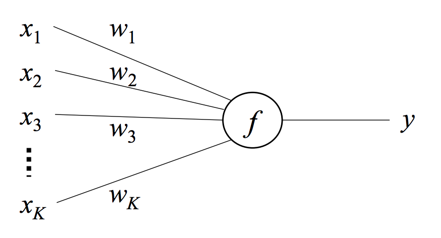
A neuron is a function that maps an input vector \(\vec x \in \mathbb{R}^K\) to a scalar output \(y\) via a weight vector \(\vec \omega \in \mathbb{R}^K\) and an activation function \(f\):

$$y = f(\vec \omega \vec x)$$

Suppose we choose a logistic function as \(f\):

$$f(u) = \frac{1}{1+e^{-u}}$$

Then, the relationship between \(\vec x\) and \(y\) becomes:

$$y = \frac{1}{1+e^{-\vec \omega \vec x}}$$

The gradient of the single neuron

Suppose we use the squared loss to update the model:

$$\text{loss} = \frac{1}{2}(t - y)^2$$

Then the gradient of the loss with respect to the parameters \(\vec \omega\) can be calculated as follows:

$$\frac{\partial \text{loss}}{\partial y} = y - t \\ \frac{\partial y}{\partial u} = \frac{\partial f(u)}{\partial u} = f(u)(1 - f(u)) \\ \frac{\partial u}{\partial \omega_i} = x_i \\ \frac{\partial \text{loss}}{\partial \omega_i} = \frac{\partial \text{loss}}{\partial y} \frac{\partial y}{\partial u} \frac{\partial u}{\partial \omega_i} = (y - t) f(u)(1 - f(u)) x_i = (y - t) y(1 - y) x_i$$

It is the result of applying the chain rule.

A fully connected layer

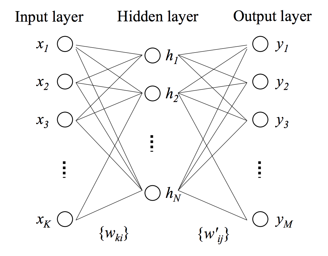
Now, let’s see a three layer neural network, which is composed by two fully connected layers. For the left fc layer, its input is a vector \(\in \mathbb{R}^K\), output is a vector \(\in \mathbb{R}^N\), and the layer parameter is a \(K \times N\) matrix. For the second layer, its input is a vector \(\in \mathbb{R}^N\), output is a vector \(\in \mathbb{R}^M\), and the layer parameter is an \(N \times M\) matrix.

In a fully connect layer, every input neuron contributes to every output neuron, and the activation function is the identity function \(f(u) = u\).

That means:

$$h_i = f(\vec \omega_i \vec x) = \vec \omega_i \vec x$$

and

$$y_i = f(\vec \omega'_i \vec h) = \vec \omega'_i \vec h$$

And the derivative is simply \(\frac{\partial f(u)}{\partial u} = 1\).

If we use some non-linear function instead of the identity function, it will give us some other layer. Suppose in all following layers, the input is a vector \(\vec x \in \mathbb{R}^N\), and the output layer is a vector \(\vec y \in \mathbb{R}^M\), thus the parameter is an \(N \times M\) matrix.

The sigmoid layer

In the sigmoid layer, the activation function is the logistic function \(f(u) = \frac{1}{1+e^{-u}}\), where

$$y_i = f(\vec \omega_i \vec x) = \frac{1}{1+e^{-\vec \omega_i \vec x}}$$

And the derivative of the logistic function is

$$\frac{\partial f(u)}{\partial u} = \frac{\partial \frac{1}{1+e^{-u}}}{\partial u} = -\frac{-e^{-u}}{(1+e^{-u})^2} = \frac{1}{1+e^{-u}}(\frac{1 + e^{-u} - 1}{1+e^{-u}} = f(u)(1 - f(u))$$

The tanh layer

In the tanh layer, we use the tanh function \(f(u) = \tanh(u) = frac{e^u - e^{-u}}{e^u + e^{-u}}\) instead.

$$y_i = f(\vec \omega_i \vec x) = \tanh(\vec \omega_i \vec x)$$

And the derivative of the tanh function is

$$\frac{\partial f(u)}{\partial u} = 1 - \tanh^2(f(u))$$

The ReLU layer

In the ReLU layer, we use the rectified linear unit function \(f(u) = \begin{cases}u \text{ if } u > \epsilon\\ 0 \text{ otherwise}\end{cases} \), where \(\epsilon\) is some positive small value or simply \(0\):

$$y_i = f(\vec \omega_i \vec x) = \begin{cases} \vec \omega_i \vec x &\text{ if } \vec \omega_i \vec x > \epsilon\\ 0 &\text{ otherwise}\end{cases}$$

And the derivative of the ReLU is

$$\frac{\partial f(u)}{\partial u} = \begin{cases}1 &\text{ if } u > \epsilon\\ 0 &\text{ otherwise}\end{cases}$$

The backward error propagation algorithm

Now let’s discuss the backpropagation algorithm. As shown in the below figure, it is a neural network with two layers. The first layer’s input is a vector \(\in \mathbb{R}^K\), output is a vector \(\in \mathbb{R}^N\), and the activation function is \(f(u)\). The second layer is a softmax regression layer, whose input is a vector \(\in \mathbb{R}^N\) and output is a vector \(\in \mathbb{R}^M\).

Where we have:

$$h_i = f(\vec \omega_i \vec x)$$

and

$$y_i = \frac{e^{\vec \omega'_i \vec h}}{Z(\vec h)}$$

where

$$Z(\vec h) = \sum_{i = 1}^M e^{\vec \omega'_i \vec h}$$

From the previous post, if we take the cross entropy as the loss, then the gradients of the loss is:

$$\frac{\partial \text{loss}}{\partial \omega'_{ij}} = (y_i - t_i) h_j$$

and

$$\frac{\partial \text{loss}}{\partial h_j} = \sum_{i=1}^M (y_i - t_i) \omega'_{ij}$$

Note that in the above equation, we already apply the reverse mode differentiation to obtain the \(\frac{\partial \text{loss}}{\partial h_j}\). In the following steps, we will further apply the reverse mode differentiation to derive the derivatives with respect to \(x_i\) and \(\omega_{ij}\).

\(\frac{\partial \text{loss}}{\partial \omega’_{ij}}\) is used to update \(\Omega’\), \(\frac{\partial \text{loss}}{\partial h_j}\) is used to propagate the contribution of the error back to the previous layer. In plain words, it is used for the reverse mode differentiation to calculate derivatives with respect to the nodes in the previous layers.

By applying the chain rule, we have:

$$\frac{\partial \text{loss}}{\partial \omega_{ki}} = \frac{\partial \text{loss}}{\partial h_i}\frac{\partial h_i}{\partial u}\frac{\partial u}{\omega_{ki}} = \frac{\partial \text{loss}}{\partial h_i} f'(h_i) x_k$$

According to the reverse mode differentiation, the derivative with respect to a node is the sum of the product over all paths. Now that, we have already calculated the derivatives with respect to all nodes in the hidden layer, we can further calculate the derivatives with respect to \(x_k\) as:

$$\frac{\partial \text{loss}}{\partial x_k} = \sum_{i=1}^N \frac{\partial \text{loss}}{\partial h_i} \frac{\partial h_i}{\partial u} \frac{\partial u}{\partial x_k} = \sum_{i=1}^N \frac{\partial \text{loss}}{\partial h_i} f'(h_i) \omega_{ki}$$

In this case, it is not necessary to calculate this quantity, as there exists no previous layers. It is listed here as an example, and the process to calculate \(\frac{\partial \text{loss}}{\partial h_j}\) is similar.

Also note that the gradients of sigmoid and tanh reduce exponentially back through the network, which will easily cause the problem of vanishing of gradient. It means that the network will fail to update the parameters. On the other hand, the ReLU does not have such kind of problem.

In summary, with the help of chain rule and reverse mode differentiation, we can derive the gradients very easily as long as we know the derivative of each basic component in the network.