When we use gradient descent methods to optimize some objective function, we need to calculate the partial derivatives of the objective function with respect to the parameters. There are ways to calculate those derivatives: the numerical differentiation, the forward-mode differentiation, and the reverse-mode differentiation (the reverse-mode automatic differentiation).
The numerical differentiation
The formulae of the numerical differentiation is easy to get by directly applying the definition of derivative:
As a result, we can approximate the derivative of \(f(\vec x)\) at \(\vec x_0\) with respect to \(x_i\) as
where \(\epsilon\) is a small positive number, and \(\vec e_i\) is a unit vector in the \(i^{th}\) direction.
The ARIMA algorithm implemented in R is optimized with such method.
When there exist great amount of parameters and evaluation of \(f(x)\) is not that cheap, this method may lead to very bad efficiency, as it has to calculate \(f(\vec x_0 + \epsilon \vec e_i)\) for every parameter in every iteration. It is very easy for a deep neural network having hundreds of thousands of parameter, which makes it impractical to use this method to calculate derivatives in optimization.
The computational graph
Before talking about the forward-mode differentiation and the reverse-mode differentiation, I will first introduce the computational graph.
Let’s consider the following expression:
where \(e\), \(a\), and \(b\) are variables. It composes the computational graph as shown below:
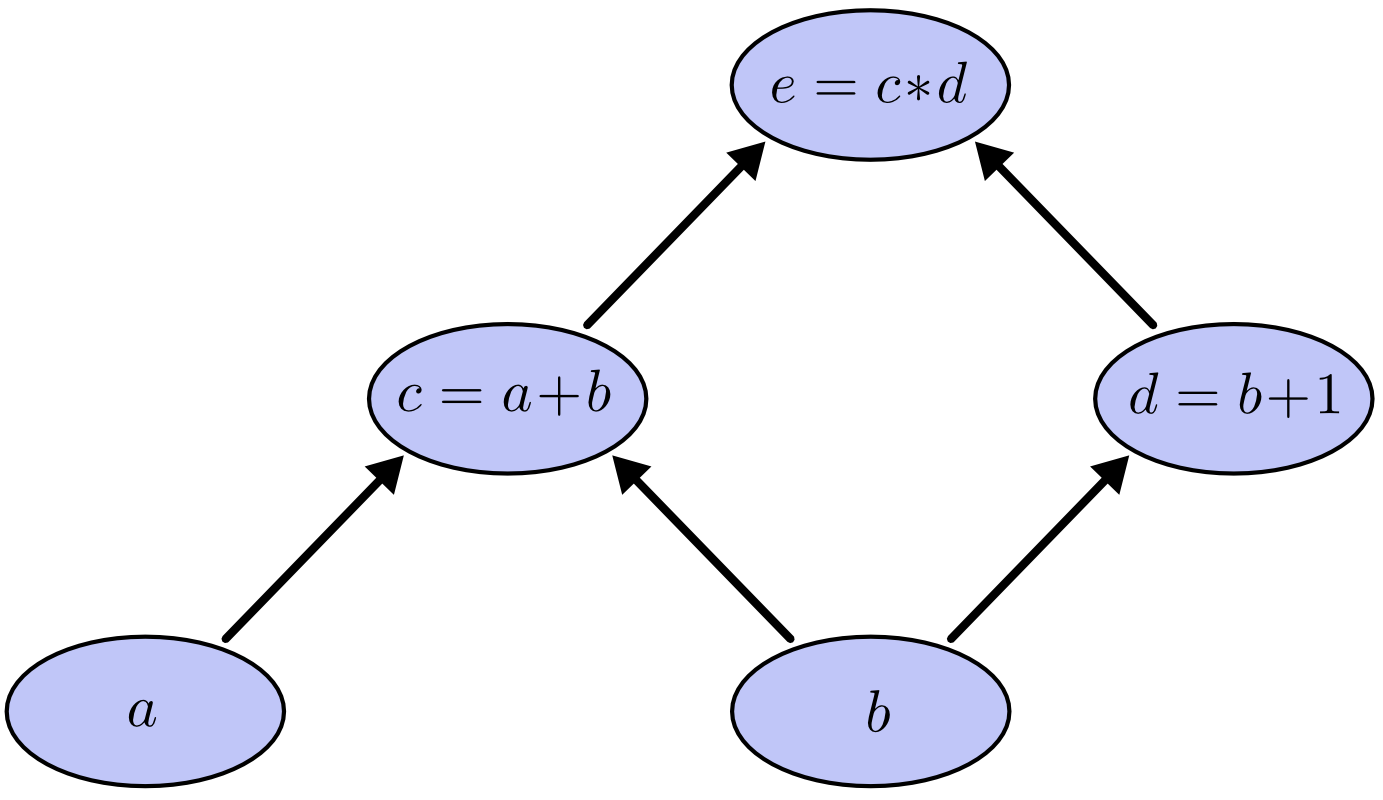
In the computational graph, \(c\) and \(d\) are two intermediary variables, or can be seen as two functions of \(a\) and \(b\).
By assigning some values to the input variables, \(a\) and \(b\) in this example, moving with the arrows will finally give us the evaluated value of the expression.
Derivatives on the computational graph
By labelling the edges of the computational graph with the partial derivatives (with the fixed input variables), we get:
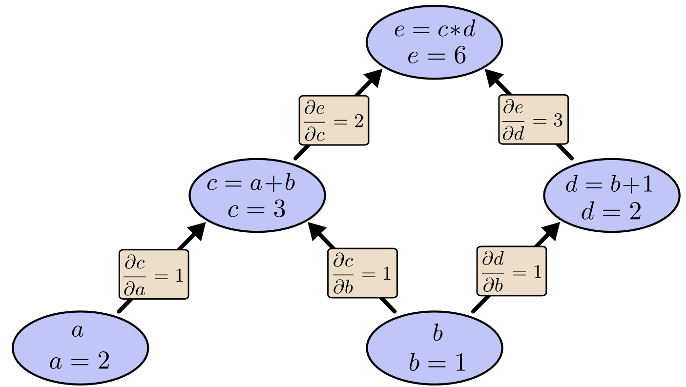
To understand what does this diagram mean, let’s take the path \(\frac{\partial{c}}{\partial{a}}\) and \(\frac{\partial{e}}{\partial{c}}\) as example.
\(\frac{\partial{c}}{\partial{a}}\) means that a variation of \(\Delta\) in \(a\) will cause a variation of \(\frac{\partial{c}}{\partial{a}}\Delta\) in \(c\). Similar for \(\frac{\partial{e}}{\partial{c}}\). Chaining the relation together, we get that a variation of \(\Delta\) in \(a\) will cause a variation of \(\frac{\partial{e}}{\partial{c}}\frac{\partial{c}}{\partial{a}}\Delta\) in \(e\).
Similarly, a variation of \(\Delta\) in \(b\) will cause a variation of \((\frac{\partial{e}}{\partial{c}}\frac{\partial{c}}{\partial{b}} + \frac{\partial{e}}{\partial{d}}\frac{\partial{d}}{\partial{b}})\Delta\) in \(e\).
In summary, in the computational graph, the derivative of a variable \(v_1\) with respect to another variable \(v_2\) equals the sum of the products of all the possible paths from \(v_2\) to \(v_1\).
The forward-mode differentiation
In the forward-mode differentiation, we calculate the relation of by changing some input variable with \(\Delta\) will cause how much variation in the output variable forwards the arrows in the graph.
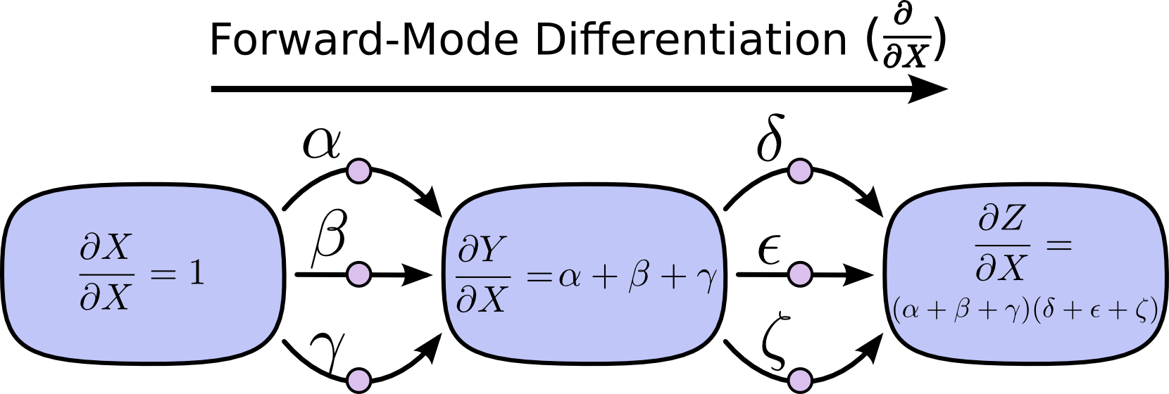
In order to compute the derivative of the output variable with respect to an input variable under current condition, we need to walk through all the paths from the input variable to the output variable.
In the case of gradient descent, we need to calculate the partial derivatives to all the parameters. For each parameter, we need to calculate
the derivative of every related node with respect to this parameter in the graph to finally get the derivative of the objective function with
respect this parameter. It is clear the graph will be passed with the number proportional to the amount of parameters in every iteration,
which is similar to the numerical differentiation. As a result, it is computational heavy.
The reverse-mode differentiation
As its name implied, in the reverse-mode differentiation, we move backwards in the graph.
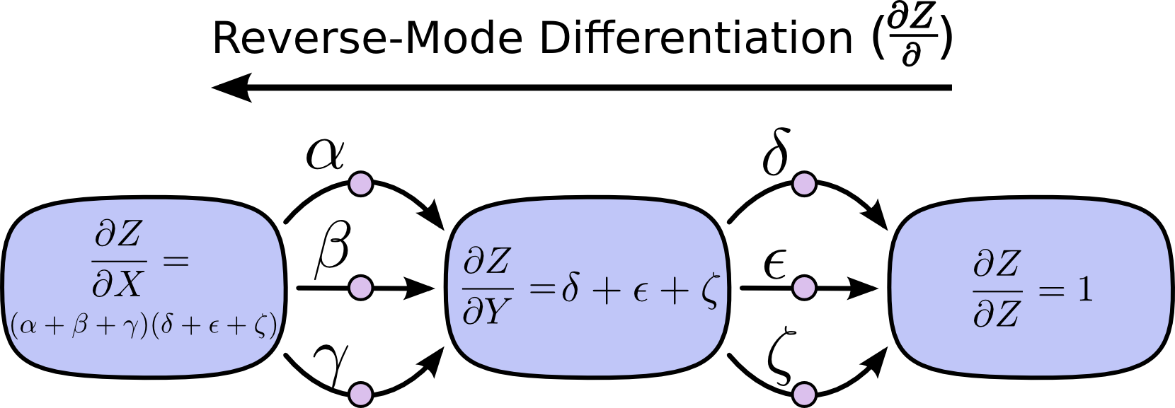
Unlike the forward-mode applying the \(\frac{\partial \cdot}{\partial x}\) operator to all the nodes, it applies the \(\frac{\partial x}{\partial \cdot}\) operator to all the nodes.
As a result, we just need to pass the computational graph twice to get all the gradients, one forward pass for computing the values of the edges in the graph, one backward pass for computing the derivatives of the output variable with respect to every node in the graph.
