Notes On Expectation Maximization And Variational Methods

Bayesian Networks

A Bayesian network is a probabilistic graphical model that represents a set of random variables and their conditional dependencies via a directed acyclic graph.

A Bayesian network is a complete model for the variables and their relationship. It can be used to answer probabilistic queries about them. For example, the network can be used to find out updated knowledge of the state of a subset of variables when other variables are observed. This process of computing the posterior distribution of variables given evidence is called probabilistic inference. The posterior gives a universal sufficient statistic for detection applications, when one wants to choose values for the variable subset which minimize some expected loss function.

In order to fully specify the Bayesian network and thus fully represent the joint probability distribution, it is necessary to specify for each node \(X\) the probability distribution for \(X\) conditional upon \(X\)’ parents. The distribution of \(X\) conditional upon its parents may have any form. Often there conditional distributions include parameters which are unknown and must be estimated from data, sometimes using the maximum likelihood approach. Direct maximization of the likelihood (or of the posterior probability) is often complex when there are unobserved variables. A classical approach to this problem is the expectation-maximization algorithm which alternates computing expected values of the unobserved variables conditional on observed data, with maximizing the complete likelihood (or posterior) assuming that previously computed expected values are correct.

A more fully Bayesian approach to parameters is to treat parameters as additional unobserved variables and to compute a full posterior distribution over all nodes conditional upon observed data, then to integrate out the parameters. This approach can be expensive and lead to large dimension models.

Expectation Maximization

Given visible variables \(\boldsymbol{y}\), hidden variables \(\boldsymbol{x}\) and model parameter \(\boldsymbol{\theta}\), maximizing the likelihood w.r.t. \(\boldsymbol{\theta}\):

$$\mathcal{L}(\boldsymbol{\theta}) = \log p(\boldsymbol{y}|\boldsymbol{\theta}) = \log \int p(\boldsymbol{x}, \boldsymbol{y} | \boldsymbol{\theta}) d \boldsymbol{x}$$

which is the marginal for the visibles written in terms of the integral over the joint distribution for hidden and visible varialbes.

Using Jensen’s inequality, any distribution over hidden variables \(q(\boldsymbol{x})\) gives

$$\mathcal{L}(\boldsymbol{\theta}) = \log \int q(\boldsymbol{x}) \frac{p(\boldsymbol{x}, \boldsymbol{y} | \boldsymbol{\theta})}{q(\boldsymbol{x})} d \boldsymbol{x} \geq \int q(\boldsymbol{x}) \log \frac{p(\boldsymbol{x}, \boldsymbol{y}|\boldsymbol{\theta})}{q(\boldsymbol{x})} d \boldsymbol{x} = \mathcal{F}(q(\boldsymbol{x}), \boldsymbol{\theta})$$

defining the \(\mathcal{F}(q(\boldsymbol{x}), \boldsymbol{\theta})\) functional, which is a lower bound on the log-likelihood.

In the EM, we alternatively optimize \(\mathcal{F}(q(\boldsymbol{x}), \boldsymbol{\theta})\) w.r.t. \(q(\boldsymbol{x})\) and \(\boldsymbol{\theta}\), and we can prove that this will never decrease \(\mathcal{L}(\boldsymbol{\theta})\).

The lower bound on the log-likelihood:

$$\mathcal{F}(q(\boldsymbol{x}), \boldsymbol{\theta}) = \int q(\boldsymbol{x})\log\frac{p(\boldsymbol{x}, \boldsymbol{y}|\boldsymbol{\theta})}{q(\boldsymbol{x})} d \boldsymbol{x} = \int q(\boldsymbol{x})\log p(\boldsymbol{x}, \boldsymbol{y}|\boldsymbol{\theta}) d \boldsymbol{x} + \mathcal{H}(q(\boldsymbol{x}))$$

where \(\mathcal{H}(q(\boldsymbol{x})) = -\int q(\boldsymbol{x})\log q(\boldsymbol{x})d\boldsymbol{x}\) is the entropy of \(q(\boldsymbol{x})\).

• E step: maximize \(\mathcal{F}(q(\boldsymbol{x}), \boldsymbol{\theta})\) w.r.t. distribution over hidden variables given the parameters:

  $$q^{(k)}(\boldsymbol{x}) := \arg\max_{q(\boldsymbol{x})} \mathcal{F}(q(\boldsymbol{x}), \boldsymbol{\theta}^{(k-1)})$$

  where we have

  $$\begin{align*} \mathcal{F}(q(\boldsymbol{x}), \boldsymbol{\theta}) &= \int q(\boldsymbol{x})\log\frac{p(\boldsymbol{x}, \boldsymbol{y}|\boldsymbol{\theta})}{q(\boldsymbol{x})} d \boldsymbol{x} \\ &= \int q(\boldsymbol{x})\log\frac{p(\boldsymbol{y} | \boldsymbol{\theta}) p(\boldsymbol{x} | \boldsymbol{y}, \boldsymbol{\theta})}{q(\boldsymbol{x})} d \boldsymbol{x} \\ &= \int q(\boldsymbol{x})\log p(\boldsymbol{y} | \boldsymbol{\theta}) d \boldsymbol{x} + \int q(\boldsymbol{x})\log\frac{p(\boldsymbol{x} | \boldsymbol{y}, \boldsymbol{\theta})}{q(\boldsymbol{x})} d \boldsymbol{x} \\ &= \log p(\boldsymbol{y} | \boldsymbol{\theta}) \int q(\boldsymbol{x}) d \boldsymbol{x} - \left(-\int q(\boldsymbol{x})\log\frac{p(\boldsymbol{x} | \boldsymbol{y}, \boldsymbol{\theta})}{q(\boldsymbol{x})} d \boldsymbol{x}\right) \\ &= \log p(\boldsymbol{y} | \boldsymbol{\theta}) - \text{KL}(q(\boldsymbol{x}), p(\boldsymbol{x}|\boldsymbol{y}, \boldsymbol{\theta})) \\ &= \mathcal{L}(\boldsymbol{\theta}) - \text{KL}(q(\boldsymbol{x}), p(\boldsymbol{x}|\boldsymbol{y}, \boldsymbol{\theta})) \end{align*}$$

  The KL divergence is non-negative and zero if and only if \(q(\boldsymbol{x}) = p(\boldsymbol{x}|\boldsymbol{y}, \boldsymbol{\theta})\).

  Thus, with fixed \(\boldsymbol{\theta}^{(k-1)}\), we achieve the maximum value of the lower bound \(\mathcal{F}(q(\boldsymbol{x}), \boldsymbol{\theta})\) when \(q^{(k)}(\boldsymbol{x}) = p(\boldsymbol{x}|\boldsymbol{y}, \boldsymbol{\theta}^{(k-1)})\).

• M step: maximize \(\mathcal{F}(q(\boldsymbol{x}), \boldsymbol{\theta})\) w.r.t. the parameters given the hidden distribution:

  $$\boldsymbol{\theta}^{(k)} := \arg\max_{\boldsymbol{\theta}} \mathcal{F}(q(\boldsymbol{x}), \boldsymbol{\theta}) = \arg\max_{\boldsymbol{\theta}} \int q^{(k)}(\boldsymbol{x})\log p(\boldsymbol{x}, \boldsymbol{y}|\boldsymbol{\theta})d\boldsymbol{x}$$

  which is equivalent to optimizing the expected complete-data likelihood \(p(\boldsymbol{x},\boldsymbol{y}|\boldsymbol{\theta})\), since the entropy of \(q(\boldsymbol{x})\) does not depend on \(\boldsymbol{\theta}\).

The difference between the log-likelihood and the bound:

$$\begin{align*} \mathcal{L}(\boldsymbol{\theta}) - \mathcal{F}(q(\boldsymbol{x}), \boldsymbol{\theta}) &= \log p(\boldsymbol{y}|\boldsymbol{\theta}) - \int q(\boldsymbol{x})\log\frac{p(\boldsymbol{x}, \boldsymbol{y}|\boldsymbol{\theta})}{q(\boldsymbol{x})}d\boldsymbol{x}\\ &= \log p(\boldsymbol{x}|\boldsymbol{\theta}) - \int q(\boldsymbol{x})\log\frac{p(\boldsymbol{x}, \boldsymbol{y}|\boldsymbol{\theta})}{q(\boldsymbol{x})}d\boldsymbol{x}\\ &= -\int q(\boldsymbol{x})\log\frac{p(\boldsymbol{x}, \boldsymbol{y}|\boldsymbol{\theta})}{q(\boldsymbol{x})}d\boldsymbol{x}\\ &= \text{KL}(q(\boldsymbol{x}), p(\boldsymbol{x}|\boldsymbol{y}, \boldsymbol{\theta})) \end{align*}$$

Although we are working with a bound on the likelihood, the likelihood is non-decreasing in every iteration:

$$\mathcal{L}(\boldsymbol{\theta}^{(k-1)}) \underset{\text{E step}}{=} \mathcal{F}(q^{(k)}(\boldsymbol{x}), \boldsymbol{\theta}^{(k-1)}) \underset{\text{M step}}{\leq} \mathcal{F}(q^{(k)}(\boldsymbol{x}), \boldsymbol{\theta}^{(k)}) \underset{\text{Jensen}}{\leq} \mathcal{L}(\boldsymbol{\theta}^{(k)})$$

Usually EM converges to a local optimum of \(\mathcal{L}(\boldsymbol{\theta})\). (of course, there are exceptions.)

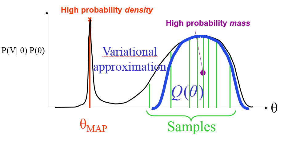
Variational Approximations

Let’s first reform EM in the case where \(\boldsymbol{x}\) is discrete: to maximize likelihood \(\ln p(\boldsymbol{y}|\boldsymbol{\theta})\), any distribution \(q(\boldsymbol{x})\) over the hidden variables defines a lower bound on \(\ln p(\boldsymbol{y}|\boldsymbol{\theta})\).

$$\ln p(\boldsymbol{y}|\boldsymbol{\theta}) \geq \sum_{\boldsymbol{x}} q(\boldsymbol{x})\ln\frac{p(\boldsymbol{x},\boldsymbol{y}|\boldsymbol{\theta})}{q(\boldsymbol{x})}=\mathcal{F}(q(\boldsymbol{x}), \boldsymbol{\theta})$$

The key difference in the variational approximations is to constrain \(q(\boldsymbol{x})\) to be of a particular tractable form, a family of variational distribution, and maximize \(\mathcal{F}\) subject to this constraint.

• E step: maximize \(\mathcal{F}(q(\boldsymbol{x}), \boldsymbol{\theta})\) w.r.t. \(q(\boldsymbol{x})\) with \(\boldsymbol{\theta}\) fixed, subject to subject to the constraint on \(q(\boldsymbol{x})\), equivalently minimize:

$$\ln p(\boldsymbol{y}|\boldsymbol{\theta}) - \mathcal{F}(q(\boldsymbol{x}), \boldsymbol{\theta}) = \sum_{\boldsymbol{x}}q(\boldsymbol{x})\ln\frac{q(\boldsymbol{x})}{p(\boldsymbol{x}|\boldsymbol{y},\boldsymbol{\theta})} = \text{KL}(q || p)$$

• M step: maximize \(\mathcal{F}(q(\boldsymbol{x}), \boldsymbol{\theta})\) w.r.t. \(\boldsymbol{\theta}\) with \(q(\boldsymbol{x})\) fixed (related to mean-field approximations)

Use Bayesian Occam’s Razor to learn model structure

Supppose in a task, the model has \(m\) classes, in order to do model selection w.r.t. best \(m\), we solve for \(m\) that gives the highest probability given data \(\boldsymbol{y}\):

$$p(m|\boldsymbol{y}) = \frac{p(\boldsymbol{y}|m)p(m)}{p(\boldsymbol{y})}$$ $$p(\boldsymbol{y}|m) = \int p(\boldsymbol{y}|\boldsymbol{\theta},m)p(\boldsymbol{\theta}|m)d\boldsymbol{\theta}$$

Interpretation of the marginal likelihood (evidence) is the probability that randomly selected parameters from the prior would generate \(\boldsymbol{y}\).

The presence of the latent variables results in additional dimensions that need to be marginalized out:

$$p(\boldsymbol{y}|m) = \int\int p(\boldsymbol{y},\boldsymbol{x}|\boldsymbol{\theta},m)p(\boldsymbol{\theta}|m)d\boldsymbol{x}d\boldsymbol{\theta}$$

The likelihood term can be complicated. There are following practical approaches to evaluate it:

• Laplace approximiations
• Large sample approximations (BIC)
• MCMC
• Variational approximations

With variational approximations, we are lower bounding the marginal likelihood:

$$\ln p(\boldsymbol{y}|m) = \ln\int p(\boldsymbol{y},\boldsymbol{x},\boldsymbol{\theta}|m)d\boldsymbol{x}d\boldsymbol{\theta} = \ln\int q(\boldsymbol{x},\boldsymbol{\theta})\frac{p(\boldsymbol{y},\boldsymbol{x},\boldsymbol{\theta}|m)}{q(\boldsymbol{x},\boldsymbol{\theta})}d\boldsymbol{x}d\boldsymbol{\theta} \geq \int q(\boldsymbol{x},\boldsymbol{\theta})\ln\frac{p(\boldsymbol{y},\boldsymbol{x},\boldsymbol{\theta}|m)}{q(\boldsymbol{x},\boldsymbol{\theta})}d\boldsymbol{x}d\boldsymbol{\theta}$$

Using a simpler, factorised approximation to \(q(\boldsymbol{x},\boldsymbol{\theta}) \approx q_x(\boldsymbol{x})q_\theta(\boldsymbol{\theta})\):

$$\ln p(\boldsymbol{y}|m) \geq \int q_x(\boldsymbol{x})q_\theta(\boldsymbol{\theta})\ln\frac{p(\boldsymbol{y},\boldsymbol{x},\boldsymbol{\theta}|m)}{q_x(\boldsymbol{x})q_\theta(\boldsymbol{\theta})}d\boldsymbol{x}d\boldsymbol{\theta} = \mathcal{F}_m(q_x(\boldsymbol{x}), q_\theta(\boldsymbol{\theta}), \boldsymbol{y})$$

Variational Bayesian learning

Maximizing the above lower bound \(\mathcal{F}_m\) leads to EM-like iterative updates:

• E-like step:

$$q_x^{(t+1)}(\boldsymbol{x}) \propto \exp\left[\int\ln p(\boldsymbol{x},\boldsymbol{y}|\boldsymbol{\theta},m)q_\theta^{(t)}(\boldsymbol{\theta})d\boldsymbol{\theta}\right]$$

• M-like step:

$$q_\theta^{(t+1)}(\boldsymbol{\theta}) \propto p(\boldsymbol{\theta}|m)\exp\left[\int\ln p(\boldsymbol{x},\boldsymbol{y}|\boldsymbol{\theta},m)q_x^{(t+1)}(\boldsymbol{x})d\boldsymbol{x}\right]$$

Maximizing \(\mathcal{F}_m\) is equivalent to minimizing KL divergence between the approximate posterior \(q_\theta(\boldsymbol{\theta})q_x(\boldsymbol{x})\) and the true posterior \(p(\boldsymbol{\theta},\boldsymbol{x}|\boldsymbol{y},m)\):

$$\ln p(\boldsymbol{y}|m) - \mathcal{F}_m(q_x(\boldsymbol{x}),q_\theta(\boldsymbol{\theta}),\boldsymbol{y}) = \int q_x(\boldsymbol{x})q_\theta(\boldsymbol{\theta})\ln\frac{q_x(\boldsymbol{x})q_\theta(\boldsymbol{\theta})}{p(\boldsymbol{\theta}, \boldsymbol{x}|\boldsymbol{y},m)}d\boldsymbol{x}d\boldsymbol{\theta} = \text{KL}(q || p)$$

Assume \(\boldsymbol{Q}\) factories \(\boldsymbol{Q(H)} = \prod_i Q_i(H_i)\), the optimal solution for one factor is given by:

$$\ln Q_i^*(H_i) = <\ln p(\boldsymbol{H}, \boldsymbol{V})>_{j \neq i} + \text{const}$$

where \(\boldsymbol{V}\) denote observed variables and \(\boldsymbol{H}\) denote hidden variables including parameters and latent variables.

Compared with EM for MAP

EM for MAP	Variational Bayesian EM
Goal: maximize \(p(\boldsymbol{\theta}|\boldsymbol{y},m)\) w.r.t. \(\boldsymbol{\theta}\)	Goal: lower bound \(p(\boldsymbol{y}|m)\)
E step: Compute \(q_x^{(t+1)}(\boldsymbol{x})=p(\boldsymbol{x}|\boldsymbol{y},\boldsymbol{\theta}^{(t)})\)	VB-E step: compute \(q_x^{(t+1)}(\boldsymbol{x})=p(\boldsymbol{x}|\boldsymbol{y},\bar{\boldsymbol{\phi}}^{(t)})\)
M step: \(\boldsymbol{\theta}^{t+1} = \arg\max\limits_{\boldsymbol{\theta}}\int q_x^{(t+1)}(\boldsymbol{x})\ln p(\boldsymbol{x},\boldsymbol{y},\boldsymbol{\theta})d\boldsymbol{x}\)	VB-M step: \(q_\theta^{(t+1)}(\boldsymbol{\theta}) \propto \exp \left[\int q_x^{(t+1)}(\boldsymbol{x})\ln p(\boldsymbol{x},\boldsymbol{y},\boldsymbol{\theta})d\boldsymbol{x}\right]\)

It has following properties:

• Reduces to the EM if \(q_\theta(\boldsymbol{\theta}) = \delta(\boldsymbol{\theta} - \boldsymbol{\theta}^*)\)
• \(\mathcal{F}_m\) increases monotonically, and incorporates the model complexity penaly
• VB-E step has the same complexity as corresponding E step
• we can use junction tree, belief propagation, Kalman filter, etc algorithms in the VB-E step, but using expected natural parameters \(\bar{\boldsymbol{\phi}}\)

Conjugate-Exponential models

The conjugate-exponential models follows two conditions:

1. The joint probability over variables is in the exponential families:

$$p(\boldsymbol{x}, \boldsymbol{y} | \boldsymbol{\theta}) = f(\boldsymbol{x}, \boldsymbol{y}) g(\boldsymbol{\theta}) \exp\{\boldsymbol{\phi(\theta)}^T\boldsymbol{u(x,y)}\}$$

where \(\boldsymbol{\phi(\theta)}\) is the vector of natural parameters, \(\boldsymbol{u(x, y)}\) are sufficient statistics.

1. The prior over parameters is conjugate to this joint probability:

$$p(\boldsymbol{\theta}| \eta, \boldsymbol{\upsilon}) = h(\eta, \boldsymbol{\upsilon}) g(\boldsymbol{\theta})^\eta \exp\{\boldsymbol{\phi(\theta)}^T\boldsymbol{\upsilon}\}$$

where \(\eta\) and \(\boldsymbol{\upsilon}\) are hyperparameters of the prior.

Conjugate priors are computationally convenient and have an intuitive interpretation:

• \(\eta\): number of pseudo-observations
• \(\boldsymbol{\upsilon}\): value of pseudo-observations

Annealed Importance Sampling (AIS)

AIS is a state-of-the-art method for estimating marginal likelihood, by breaking a difficult integral into a series of easier ones. It combines the ideas from importance sampling, Markov chain Monte Carlo and annealing:

Define \(Z_k = \int d\boldsymbol{\theta} p(\boldsymbol{\theta}|m)p(\boldsymbol{y}|\boldsymbol{\theta}, m)^{\tau(k)} = \int d\boldsymbol{\theta}f_k(\boldsymbol{\theta})\)

with \(\tau(0) = 0 \Rightarrow Z_0 = \int d\boldsymbol{\theta} p(\boldsymbol{\theta}|m) = 1 \leftarrow \text{normalisation factor}\)

with \(\tau(K) = 1 \Rightarrow Z_K = p(\boldsymbol{y}|m) \leftarrow \text{marginal likelihood}\)

and we have \(\frac{Z_K}{Z_0} = \frac{Z_1}{Z_0} \cdot \frac{Z_2}{Z_1} \cdots \frac{Z_K}{Z_{K-1}}\)

To importance sample from \(f_{k-1}(\boldsymbol{\theta})\):

$$\frac{Z_k}{Z_{k-1}} \equiv \int d\boldsymbol{\theta} \frac{f_k(\boldsymbol{\theta})}{f_{k-1}(\boldsymbol{\theta})}\frac{f_{k-1}(\boldsymbol{\theta})}{Z_{k-1}} \approx \frac{1}{R}\sum\nolimits_{r=1}{R}\frac{f_k(\boldsymbol{\theta}^{(r)})}{f_{k-1}(\boldsymbol{\theta}^{(r)})} = \frac{1}{R} \sum\nolimits_{r=1}^R p(\boldsymbol{y}|\boldsymbol{\theta}^{(r)}, m)^{\tau(k) - \tau(k-1)}$$

with \(\boldsymbol{\theta}^{(r)} \sim f_{k-1}(\boldsymbol{\theta})\)

Variational Inference v.s. ML/MAP

Supppose in a Bayesian network, we have observed variables \(\boldsymbol{V}\) and hidden variables \(\boldsymbol{H}\), with \(\boldsymbol{H}\) including parameters and latent variables, the learning/inference process involves finding \(P(H_1, H_2, \cdots | \boldsymbol{V})\).

$$P(\boldsymbol{\theta}|\boldsymbol{V}) = \frac{P(\boldsymbol{V}|\boldsymbol{\theta})P(\boldsymbol{\theta})}{P(\boldsymbol{V})} \propto P(\boldsymbol{V}|\boldsymbol{\theta})P(\boldsymbol{\theta})$$

Variational Message Passing

VMP makes it easier and quicker to apply factorized variational inference. VMP carries out variational inference using local computations and message passing on the graphical model. Modular algorithm allows modifying, extending or combining models.

• VMP I the exponential family

  Conditional distributions expressed in exponential family form:

  $$\ln p(\boldsymbol{x} | \boldsymbol{\theta}) = \boldsymbol{\theta}^Tu(\boldsymbol{x}) + g(\boldsymbol{\theta}) + f(\boldsymbol{x})$$

  where \(\boldsymbol{\theta}\) is the natural parameter vector, and \(u(\boldsymbol{x})\) is the sufficient statistics vector.

• VMP II the conjugacy

  Parents and children are chosen to be conjugate: the same functional form.

  For instance, with \(X \rightarrow Z \leftarrow Y\), we have:

  $$\ln p(\boldsymbol{x}|\boldsymbol{\theta}) = \boldsymbol{\theta}^Tu(\boldsymbol{x}) + g(\boldsymbol{\theta}) + f(\boldsymbol{x})$$ $$\ln p(\boldsymbol{z} | \boldsymbol{x}, \boldsymbol{y}) = \phi(\boldsymbol{y}, \boldsymbol{z})^Tu(*\boldsymbol{x}) + g'(\boldsymbol{x}) + f'(\boldsymbol{y}, \boldsymbol{z})$$

  Common choices are:

  • Gaussian for the mean of a Gaussian
  • Gamma for the precision of a Gaussian
  • Dirichlet for the parameters of a discrete distribution

• VMP III the message

  Parent to child \(X \rightarrow Z\), the message is \(m_{x\rightarrow z} = <u(\boldsymbol{x})>_{Q(\boldsymbol{x})}\)

  Child to parent \(Z \rightarrow X\), the message is \(m_{z\rightarrow x} = <\phi(\boldsymbol{y}, \boldsymbol{z})>_{Q(\boldsymbol{y})Q(\boldsymbol{z})}\)

• VMP IV the update

  Optimal \(Q(\boldsymbol{x})\) has the same form as \(p(\boldsymbol{x}|\boldsymbol{\theta})\) but with updated parameter vector \(\boldsymbol{\theta}^*\):

  $$\boldsymbol{\theta}^* = <\boldsymbol{\theta}> + \sum_{j \in \text{ch}(x)} m_{j \rightarrow x}$$

  where \(<\boldsymbol{\theta}>\) is the computed messages from parents.

Link to Gibbs Sampling

For a joint density \(f(x, y_1, y_2, \cdots, y_k)\), we are interested in some features of the marginal density.

$$f(x) = \int\int\cdots\int f(x, y_1, y_2, \cdots, y_k)dy_1dy_2\cdots dy_k$$

For instance, the average \(\mathbb{E}[X] = \int xf(x) dx\).

If we can sample from the marginal distribution, then we can approximate it with \(\lim\limits_{n\to\infty}\frac{1}{n}\sum\nolimits_{i=1}^n X_i = \mathbb{E}[X]\) without using \(f(x)\) explicitly in integration.

We may take the last \(n\) \(X\)-values after many Gibbs passes \(\frac{1}{n}\sum\limits_{i=m}^{m+n}X^i \approx \mathbb{E}[X]\), or take the last value \(x_i^{n_i}\) of \(n\)-many sequences of Gibbs passes \(\frac{1}{n}\sum\limits_{i=i}^n X_i^{n_i} \approx \mathbb{E}[X]\).

In the EM, \(\mathcal{L}(\boldsymbol{\theta}; \boldsymbol{x})\) is the likelihood function for \(\boldsymbol{\theta}\) w.r.t. the incomplete data \(\boldsymbol{x}\). \(\mathcal{L}(\boldsymbol{\theta};(\boldsymbol{x},\boldsymbol{z}))\) is the likelihood function for \(\boldsymbol{\theta}\) w.r.t. the complete data \((\boldsymbol{x}, \boldsymbol{z})\). \(\mathcal{L}(\boldsymbol{\theta}; \boldsymbol{z}|\boldsymbol{x})\) is the conditional likelihood for \(\boldsymbol{\theta}\) w.r.t. \(\boldsymbol{z}\) given \(\boldsymbol{x}\), which is based on \(h(\boldsymbol{z}|\boldsymbol{x},\boldsymbol{\theta})\) the conditional density for the data \(\boldsymbol{z}\), given \(\boldsymbol{x}, \boldsymbol{\theta}\).

As \(f(\boldsymbol{x}|\boldsymbol{\theta}) = \frac{f(\boldsymbol{x}, \boldsymbol{z} | \boldsymbol{\theta})}{h(\boldsymbol{z} | \boldsymbol{x}, \boldsymbol{\theta})}\), we have:

$$\begin{equation} \log \mathcal{L}(\boldsymbol{\theta}; \boldsymbol{x}) = \log \mathcal{L}(\boldsymbol{\theta}; (\boldsymbol{x}, \boldsymbol{z})) - \log \mathcal{L}(\boldsymbol{\theta}; \boldsymbol{z}|\boldsymbol{x}) \label{eq:l} \end{equation}$$

We use the EM algorithm to compute the MLE \(\hat{\boldsymbol{\theta}} = \arg\max_{\boldsymbol{\theta}} \mathcal{L}(\boldsymbol{\theta}; \boldsymbol{x})\).

With an arbitrary choice of \(\hat{\boldsymbol{\theta}}_0\), define (E step):

$$Q(\boldsymbol{\theta}|\boldsymbol{x}, \hat{\boldsymbol{\theta}}_0) = \int h(\boldsymbol{z}|\boldsymbol{x}, \hat{\boldsymbol{\theta}}_0)\log \mathcal{L}(\boldsymbol{\theta}; \boldsymbol{x}, \boldsymbol{z}) d\boldsymbol{z}$$ $$H(\boldsymbol{\theta}|\boldsymbol{x}, \hat{\boldsymbol{\theta}}_0) = \int h(\boldsymbol{z}|\boldsymbol{x}, \hat{\boldsymbol{\theta}}_0)\log \mathcal{L}(\boldsymbol{\theta}; \boldsymbol{z}|\boldsymbol{x}) d\boldsymbol{z}$$

Then we have:

$$\log \mathcal{L}(\boldsymbol{\theta};\boldsymbol{x}) = Q(\boldsymbol{\theta}|\boldsymbol{x},\boldsymbol{\theta}_0) - H(\boldsymbol{\theta}|\boldsymbol{x}, \boldsymbol{\theta}_0)$$

As we integrated out \(\boldsymbol{z}\) from \eqref{eq:l} using the conditional density \(h(\boldsymbol{z}|\boldsymbol{x}, \hat{\boldsymbol{\theta}}_0)\).

The EM algorithm is an iteration of

1. E step: determine the integral \(Q(\boldsymbol{\theta}|\boldsymbol{x}, \hat{\boldsymbol{\theta}}_j)\)
2. M step: define \(\hat{\boldsymbol{\theta}}_{j+1}\) as \(\arg\max\limits_{\boldsymbol{\theta}} Q(\boldsymbol{\theta}|\boldsymbol{x}, \hat{\boldsymbol{\theta}}_j)\)

continue until there is convergence of the \(\hat{\boldsymbol{\theta}}_j\).

Generalized EM algorithm

Let \(p(\boldsymbol{z})\) be any distribution over the augumented data \(\boldsymbol{z}\), with density \(p(\boldsymbol{z})\).

Define

$$\mathcal{F}(\boldsymbol{\theta}, p(\boldsymbol{z})) = \int p(\boldsymbol{z})\log\mathcal{L}(\boldsymbol{\theta};\boldsymbol{x}, \boldsymbol{z})d\boldsymbol{z} - \int p(\boldsymbol{z})\log p(\boldsymbol{z}) d\boldsymbol{z} = \mathbb{E}_p\left[\log \mathcal{L}(\boldsymbol{\theta}; \boldsymbol{x}, \boldsymbol{z})\right] - \mathbb{E}_p\left[\log p(\boldsymbol{z})\right]$$

when \(p(\boldsymbol{z}) = h(\boldsymbol{z}|\boldsymbol{x}, \hat{\boldsymbol{\theta}}_0)\) from above, the \(\mathcal{F}(\boldsymbol{\theta}, p(\boldsymbol{z})) = \log\mathcal{L}(\boldsymbol{\theta}; \boldsymbol{x})\).

Claim: for a fixed (arbitrary) value \(\boldsymbol{\theta} = \hat{\boldsymbol{\theta}}_0\), \(\mathcal{F}(\hat{\boldsymbol{\theta}}_0, p(\boldsymbol{z}))\) is maximized over distribution \(p(\boldsymbol{z})\) by choosing \(p(\boldsymbol{z}) = h(\boldsymbol{z}|\boldsymbol{x},\hat{\boldsymbol{\theta}}_0)\).

Thus the EM algorithm is a sequence of M-M steps:

• the old E step now is a max over the second term in \(\mathcal{F}(\hat{\boldsymbol{\theta}}_0, p(\boldsymbol{z}))\), given the first term

• the second step remains (as in EM) a max over \(\boldsymbol{\theta}\) for a fixed second term, which does not involve \(\boldsymbol{\theta}\)

Suppose that the augumented data \(\boldsymbol{z}\) are multidimensional, consider the GEM approach and, instead of maximizing the choice of \(p(\boldsymbol{z})\) over all of the augumented data - instead of the old E step - instead maximize over only one coordinate of \(\boldsymbol{z}\) at a time, alternating with the (old) M step.

This gives the link with Gibbs algorithm: instead of maximizing at each of these two steps, use the conditional distributions, we sample from them.

Summary

EM can be interpreted as a lower bound maximization algorithm. For many models of interest the E step is intractable. For such models, an approximate E step can be used in a variational lower bound optimization algorithm. This lower bound idea also be used to do variational Bayesian learning. Bayesian learning embodies automatic Occam’s Razor via the marginal likelihood. This makes it possible to avoid overfitting and model selection.