Notes On Sampling Revisit

In previous post efficient sampling from known distribution, I have introduced how to perform sampling from a distribution. In this post, I will talk about some different kinds of sampling algorithms.

Monte Carlo Sampling

Monte Carlo sampling is often used in two kinds of problems:

• Sampling from a distribution \(p(x)\), which is often a posterior distribution
• Approximating integrals of the form \(\int f(x)p(x) dx\) by computing expectation of \(f(x)\) with density \(p(x)\).

Suppose \({x^{(i)}}\) is an i.i.d. random sample drawn from \(p(x)\). Then the strong law of large numbers has:

$$\frac{1}{N}\sum_{i=1}^N f(x^{(i)}) \stackrel{\text{a.s}}{\longrightarrow} \int f(x)p(x)dx$$

Moreover, the rate of convergence is proportional to \(\sqrt{N}\). However, the proportionality constant increases exponentially with the dimension of the integral.

Strong Law of Large Numbers

Let \(X_1\),\(X_2\),\(\cdots\) be a sequence of independent and identically distributed random variables, each having a finite mean \(\mu = \mathbb{E}(X_i)\), then with probability \(1\) we have

$$\frac{X_1 + X_2 + \cdots + X_M}{M} \rightarrow \mu \quad \text{ as } \quad M \rightarrow \infty$$

Suppose we want to draw from the posterior distribution \(p(\theta|y)\), but we cannot sample independent draws from it. For example, we do not know the normalizing constant. However we may be able to sample draws from \(p(\theta|y)\) that are slightly dependent. If we can sample slightly dependent draws using a Markov chain then we can still find quantities of interests from those draws.

Rejection Sampling

Rejection sampling is based on the observation that to sample a random variable one can perform a uniformly random sampling of a 2D cartesian graph, and keep the samples in the region under the graph of its density function. Note that this property can be extended to N-dimension functions.

Suppose we want to sample from the density \(p(x)\) as shown in bellow:

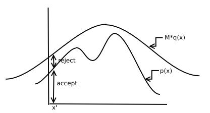
If we can sample uniformly from the 2D region under the curve, then this process is the same as sampling from \(p(x)\).

The general form of rejection sampling assumes that the board is not necessarily rectangular but is shaped according to some distribution that we know how to sample from (for example, using inversion sampling), and which is at least as high at every point as the distribution we want to sample from, so that the former completely encloses the latter.

In rejection sampling, another density \(q(x)\) is considered from which we can sample directly under the restriction that \(p(x) < M q(x)\) where \(M > 1\) is an appropriate bound on \(\frac{p(x)}{q(x)}\). The rejection sampling algorithm is described below:

$$\begin{align} &i \leftarrow 0\\ &\text{while } i \neq N \text{ do}\\ &\quad x^{(i)} \sim q(x)\\ &\quad u \sim U(0,1)\\ &\quad \text{if } u < \frac{p(x^{(i)})}{M q(x^{(i)})} \text{ then}\\ &\qquad \text{accept } x^{(i)}\\ &\qquad i \leftarrow i + 1\\ &\quad \text{else}\\ &\qquad \text{reject } x^{(i)}\\ &\quad \text{end if}\\ &\text{end while} \end{align}$$

Informally, all this process does is sampling \(x^{(i)}\) from some distribution and then it decides whether to accept it or reject. The main problem with this process is that \(M\) is generally large in high-dimensional spaces and since \(p(\text{accept}) \propto \frac{1}{M}\), rejection rate will be large.

Importance Sampling

The goal is to compute \(I(f) = \int f(x)p(x) dx\). If we have a density \(q(x)\) which is easy to sample from, we can sample \(x^{(i)} \sim q(x)\). Define the importance weight as:

$$w(x^{(i)}) = \frac{p(x^{(i)})}{q(x^{(i)})}$$

Consider the weighted Monte Carlo sum:

$$\begin{align} \frac{1}{N}\sum_{i=1}^N f(x^{(i)}) w(x^{(i)}) &= \frac{1}{N} \sum_{i=1}^N f(x^{(i)}) \frac{p(x^{(i)})}{q(x^{(i)})}\\ &\stackrel{\text{a.s}}{\rightarrow} \int (f(x)\frac{p(x)}{q(x)}) q(x) dx \\ &= \int f(x)p(x) dx \end{align}$$

In principle, we can sample from any distribution \(q(x)\). In practice, we would like to choose \(q(x)\) as close as possible to \(|f(x)|w(x)\) to reduce the variance of our estimator.

Remark 1 We do not need to know the normalization constants for \(p(x)\) and \(q(x)\). Sine \(w = \frac{p}{q}\), we can compute

$$\int f(x)p(x) dx \approx \frac{\sum_{i=1}^N f(x^{(i)})w(x^{(i)})}{\sum_{i=1}^N w(x^{(i)})}$$

where because of the ratio, the normalizing constants will cancel.

Thus, we can now compute integrals using importance sampling. However, we do not directly get samples from \(p(x)\). To get samples from \(p(x)\), we must sample from the weighted sample from our importance sampler. This process is called Sampling Importance Re-sampling, which is described below.

Now, combing back to the question of how to pick \(q(x)\). Ideally, we would like to pick \(q(x)\) such that the variance of \(f(x)w(x)\) is minimum.

$$\mathbb{Var}_{q(x)} f(x)w(x) = \mathbb{E}_{q(x)} {f(x)}^2{w(x)}^2 - {I(f)}^2$$ $$\begin{align} \mathbb{E}_{q(x)}{f(x)}^2{w(x)}^2 &\geq \quad (\mathbb{E}|f(x)|w(x))^2 (\text{Jensen's Inequality})\\ &= (\int |f(x)|p(x) dx)^2 \end{align}$$

The term \({I(f)}^2\) is independent of \(q\). So, the best \(q^*(x)\) which makes the variance minimum is given by:

$$q^*(x) = \frac{|f(x)|p(x)}{\int |f(x)|p(x) dx}$$

One with picking \(q(x)\) is that since \(p(x)\) was hard to sample from thus, \(|f(x)|p(x)\) usually would also be hard to sample from.

Sampling Importance Re-sampling

SIR is simply sampling

$$x^{(i)*} \sim \hat{p}_N(x) = \frac{1}{N} \sum_{i=1}^N w(x^{(i)})\delta_{x^{i}}(x)$$

This generates a sample from \(p(x)\) and is really just sampling with replacement from collection \({x^{(i)}}\) with probability proportional to normalized weights.

$$\hat{\hat{p}}_N (x) = \frac{1}{N} \sum_{i=1}^N \delta_{x^{(i)*}}(x)$$

Statistically, there is no advantage in working with SIR because of the introduction of variance again in re-sampling.

Markov chain Monte Carlo method

MCMC is a class of methods in which we can simulte draws that are slightly dependent and are approximately from a (posterior) distribution. In Bayesian statistics, there are generally two MCMC algorithms that we use: the Gibbs Sampler and the Metropolis-Hastings algorithm.

Markov Chain

A stochastic process in which future states are independent of past states given the present state.

Stochastic Process

A consecutive set of random (not deterministic) quantities defined on some known state space \(\Theta\).

Ergodic Theorem

Let \(\theta^{(2)}, \theta^{(2)}, \cdots, \theta^{(M)}\) be \(M\) values from a Markov chain that is aperiodic, irreducible, and positive recurrent (the the chain is ergodic) and \(\mathbb{E}[g(\theta)] < \infty\). Then with probability \(1\),

$$\frac{1}{M} \sum_{i=1}^M g(\theta_i) \rightarrow \int_{\Theta} g(\theta)\pi(\theta) d\theta$$

as \(M \rightarrow \infty\), where \(\pi\) is the stationary distribution. This is the Markov chain analog to the SLLN, and it allows us to ignore the dependence between draws of the Markov chain when we calculate quantities of interest from the draws.

A Markov chain is aperiodic if the only length of time for which the chain repeats some cycle of values is the trivial case with cycle length equal to one.

A Markov chain is irreducible if it is possible go from any state to any other state (ot necessarily in one step).

A Markov chain is recurrent if for any given state \(i\), if the chain starts at \(i\), it will eventually return to \(i\) with probability \(1\).

A Markov chain is positive recurrent if the expected return time to state \(i\) is finite; otherwise it is null recurrent.

Thinning: In order to break the dependence between draws in the Markov chain, some have suggested only keeping every \(d\)th draw of the chain.

Pros:

• Perhaps gets you a little closer to i.i.d. draws.
• Saves memory by storing a fraction of the draws.

Cons:

• Unnecessary with ergodic theorem.
• Increase the variance of the Monte Carlo estimates.

Metropolis-Hastings

The Metropolis-Hastings algorithm is a Markov chain Monte Carlo method for obtaining a sequence of random samples from a probability distribution for which direct sampling is difficult.

Suppose we have a posterior \(p(\theta|y)\) that we want to sample from, but

• the posterior doesn’t look like any distribution we know (no conjugacy)
• the posterior consists of more than 2 parameters (grid approximations intractable)
• some of the full conditionals do not look like any distributions we know (no Gibbs sampling for those whose full conditionals we don’t know)

If all else fails, we can use the Metropolis-Hastings algorithm which will always work.

The Metropolis-Hastings algorithm can draw samples from any probability distribution \(p(x)\), provided you can compute the value of a function \(f(x)\) that is proportional to the density of \(p(x)\). The lax requirement that \(f(x)\) should be merely proportional to the density, rather than exactly equal to it, makes the Metropolis-Hastings algorithm particularly useful, because calculating the necessary normalization factor is often extremely difficult in practice.

The Metropolis-Hastings algorithm works by generating a sequence of sample values in such a way that, as more and more sample values are produced, the distribution of values more closely approximates the desired distribution \(p(x)\). These sample values are produced iteratively, with the distribution of the next sample being dependent only on the current sample value (thus making the sequence of samples into a Markov chain).

Let \(f(x)\) be a function that is propotional to the desired probability distribution \(p(x)\)

1. Initialization: Choose an arbitrary point \(x_0\) to be the first sample, and choose an arbitrary probability density \(g(x|y)\) that suggests a candidate for the next sample value \(x\), given the previous sample value \(y\). For the Metropolis algorithm, \(g\) must be symmetric; in other words, it must satisfy \(g(x|y)=g(y|x)\). A usual choice is to let \(g(x|y)\) be a Gaussian distribution centered at \(y\), so that points closer to \(y\) are more likely to be visited next – making the sequence of samples into a random walk. The function \(g\) is referred to as the proposal density or jumping distribution.
2. For each iteration \(t\):
   • Generate a candidate \(x’\) for the next sample by picking from the distribution \(g(x’|x_t)\).
   • Calculate the acceptance ratio \(\alpha=\frac{f(x’)}{f(x_t)}\), which will be used to decide whether to accept or reject the candidate. Because \(f\) is propotional to the density of \(p\), we have that \(\alpha=\frac{f(x’)}{f(x_t)}=\frac{p(x’)}{p(x_t)}\).
   • If \(\alpha \geq 1\), then the candidate is more likely than \(x_t\); automatically accept the candidate by setting \(x_{t+1}=x’\). Otherwise, accept the candidate with probability \(\alpha\); if the candidate is rejected, set \(x_{t+1}=x_t\) instead.

In Metropolis-Hastings sampling, samples mostly move towards higher density regions, but sometimes also move downhill. In comparison to rejection sampling where we always throw away the rejected samples, here we sometimes keep those samples as well.

$$\begin{align} &\text{Init } x^{(0)}\\ &\text{for } i = 0 \text{ to } N-1 \text{ do}\\ &\quad u \sim U(0,1)\\ &\quad x^* \sim q(x^* | x^{(i)})\\ &\quad \text{if } u < \min\{1, \frac{p(x^*)q(x^{(i)}|x^*)}{p(x^{(i)})q(x^*|x^{(i)})}\} \text{ then}\\ &\qquad x^{(i+1)} \leftarrow x^*\\ &\quad \text{else}\\ &\qquad x^{(i+1)} \leftarrow x^{(i)}\\ &\quad \text{end if}\\ &\text{end for} \end{align}$$

Remark 2 In line 5 of the algorithm, if \(q\) is symmetric then \(\frac{q(x^{(i)}|x^*)}{q(x^*|x^{(i)})}=1\). This term was later introduced to the original Metropolis algorithm by Hastings.

Compared with an algorithm like adaptive rejection sampling that directly generates independent samples from a distribution, Metropolis-Hastings and other MCMC algorithms have a number of disadvantages:

• The samples are correlated. Even though over the long term they do correctly follow \(p(x)\), a set of nearby samples will be correlated with each other and not correctly reflect the distribution. This means that if we want a set of independent samples, we have to throw away the majority of samples and only take every \(n\)th sample, for some value of \(n\). Autocorrelation can be reduced by increaing the jumping width, but this will also increase the likehood of rejection of the proposed jump. Too large or too small a jumping size will lead to a slow-mixing Markov chain, i.e. a highly correlated set of samples, so that a very large number of samples will be needed to get a reasonable estimate of any desired property of the distribution.
• Although the Markov chain eventually converges to the desired distribution, the initial samples may follow a very different distribution, especially if the starting point is in a region of low density. As a result, a burn-in period is typically necessary, where an initial number of samples are thrown away.

As a matter of practice, most people throw out a certain number of the first draws, known as the burn-in. This is to make our draws closer to the stationary distribution and less dependent on the starting point.

Once we have a Markov chain taht has converged to the stationary distribution, then the draws in our chain appear to be like draws from \(p(\theta|y)\), so it seems like we should be able to use Monte Carlo Integration methods to find quantities of interest.

On the other hand, most simple rejection sampling methods suffer from the curse of dimensionality, where the probability of rejection increases exponentially as a function of the number of dimensions. Metropolis-Hastings, along with other MCMC methods, do not have this problem to such a degree, and thus are ofthen the only solutions available when the number of dimensions of the distribution to be sampled is high.

Gibbs Sampling

Suppose we have a joint distribution \(p(\theta_1,\cdots,\theta_k)\) that we want to sample from. We can use the Gibbs sampler to sample from the joint distribution if we knew the full conditional distributions for each parameter. For each parameter, the full conditional distribution is the distribution of the parameter conditional on the know information and all the other parameters: \(p(\theta_j|\theta_{-j},y)\).

The Hammersley-Clifford Theorem (for two blocks)

Suppose we have a joint density \(f(x,y)\). The theorem proves that we can write out the joint density in terms of the conditional densities \(f(x|y)\) and \(f(y|x)\):

$$f(x,y) = \frac{f(y|x)}{\int \frac{f(y|x)}{f(x|y)} dy}$$ $$\int \frac{f(y|x)}{f(x|y)} dy = \int \frac{\frac{f(x,y)}{f(x)}}{\frac{f(x,y)}{f(y)}} dy = \int \frac{f(y)}{f(x)} dy = \frac{1}{f(x)}$$

The Gibbs sampler is a technique for generating random variables from a (marginal) distribution indirectly, without having to calculate the density.

Suppose we are given a joint density \(f(x,y_1,y_2,\cdots,y_p)\), and are interested in obtaining characteristics of the marginal density

$$f(x) = \int\cdots\int f(x,y_1,y_2,\cdots,y_p) dy_1 dy_2 \cdots dy_p$$

such as the mean or variance. If the integration is extremely difficult to perform, the Gibbs sampler provides an alternative method for obtaining \(f(x)\).

Rather than compute or approximate \(f(x)\) directly, the Gibbs sampler allows us effectively to generate a sample \(X_1, \cdots, X_m \sim f(x)\) without requiring \(f(x)\). And we compute mean or variance based on population quantities.

In a two-variable case, the Gibbs sampler generates a sample from \(f(x)\) by sampling instead from the conditional distributions \(f(x|y)\) and \(f(y|x)\), distributions that are ofthen known in statistical models. And we generate a sequence of random variables

$$Y'_0, X'_0, Y'_1, X'_1, Y'_2, X'_2,\cdots,Y'_k,X'_k$$

The initial value \(Y’_0=y’_0\) is specified, and the rest is obtained iteratively by:

$$X'_j \sim f(x|Y'_j = y'_j)$$ $$Y'_{j+1} \sim f(y | X'_j = x'_j)$$

Under general conditions, the distribution of \(X’_k\) converges to \(f(x)\) as \(k \rightarrow \infty\).

The convergence of the Gibbs samples is a consequence of the Markovian nature of the generation iteration. In a two random variable case, the transition probability is \(A_{x|x} = f(x_{i+1}|x_i) = \sum f(x_{i+1}|y)f(y|x_i) = A_{y|x}A_{x|y}\). Thus we have \(P(X’_k=x_k | X’_0 = x_0) = (A_{x|x})^k\).

As long as all the entries of \(A_{x|x}\) are positive, then for any initial probability \(f_0\), as \(k \rightarrow \infty\), \(f_k\) converges to the unique distribution \(f\) that is a sationary point which satisfies

$$fA_{x|x} = f$$

If the Gibbs sequence converges, the \(f\) that satisfies the above equation must be the marginal distribution of \(X\).

For more than two variables, in each iteration we sample through each variable with the conditional probability. In fact, a defining characteristic of the Gibbs sampler is that it always uses the full set of univariate conditionals to define the iteration.

References

link1, link2, link3, link4, and link5