Notes On Proximal Algorithms

Much like Newton’s method is a standard tool for solving unconstrained smooth optimization problems of modest size, proximal algorithms can be viewed as an analogous tool for nonsmooth, constrained, large-scale, or distributed versions of there problems. They are generally applicable, but are especially well-suited to problems of substantial recent interest involving large or high-dimensional datasets.

Proximal methods sit at a higher level of abstraction than classical algorithms like Newton’s method: the base operation is evaluating the proximal operator of a function, which itself involves solving a small convex optimization problem. These subproblems, which generalize the problem of projecting a point onto a convex set, often admit closed-form solutions or can be solved very quickly with standard or simple specialized methods. In classical optimization algorithms, the base operations are low-level, consisting of linear algebra operations and the computation of gradients and Hessians.

Definition

Let \(f: \mathcal{R}^n \rightarrow \mathcal{R} \cup \{+\infty\}\) be a closed proper convex function, which means that its epigraph

$$\text{epi} f = \{(x, t) \in \mathcal{R}^n \times \mathcal{R} | f(x) \le t \}$$

is a nonempty closed convex set. The effective domain of \(f\) is

$$\text{dom} f = \{x \in \mathcal{R}^n | f(x) \lt +\infty \}$$

i.e. the set of points for which \(f\) takes on finite values.

The proximal operator \(\text{prox}_f : \mathcal{R}^n \rightarrow \mathcal{R}^n \) of \(f\) is defined by

$$\text{prox}_f(v) = \underset{x}{\arg\min}\left(f(x) + \frac{1}{2}||x - v||_2^2 \right)$$

where \(||\cdot||_2\) is the usual Euclidean norm. The function minimized on the righthand side is strongly convex and not everywhere infinite, so it has a unique minimizer for every \(v \in \mathcal{R}^n\) (even when \(\text{dom} f \not\subseteq \mathcal{R}^n\)).

We will often encounter the proximal operator of the scaled function \(\lambda f\), where \(\lambda \gt 0\), which can be expressed as

$$\text{prox}_{\lambda f}(v) = \underset{x}{\arg\min}\left(f(x) + \frac{1}{2\lambda}||x - v||_2^2\right)$$

This is also called the proximal operator of \(f\) with parameter \(\lambda\).

Interpretations

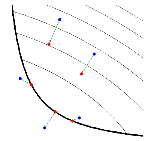
In the above picture, the thin black lines are level curves of a convex function \(f\); the thicker black line indicates the boundary of its domain. Evaluating \(\text{prox}_f\) at the blue points moves them to the corresponding red points. The three points in the domain of the function stay in the domain and move towards the minimum of the function, while the other two move to the boundary of the domain and towards the minimum of the function.

The parameter \(\lambda\) controls the extent to which the proximal operator maps points towards the minimum of \(f\), with larger values of \(\lambda\) associated with mapped points near the minimum, and smaller values giving a smaller movement towards the minimum.

The definition indicates that \(\text{prox}_f(v)\) is a point that compromises between minimizing \(f\) and being near to \(v\). For this reason, \(\text{prox}_f(v)\) is sometimes called a proximal point of \(v\) with respect to \(f\). In \(\text{prox}_{\lambda f}\), the parameter \(\lambda\) can be interpreted as a relative weight or trade-off parameter between these terms.

When \(f\) is the indicator function

$$\text{I}_\mathcal{C}(x) = \begin{cases} 0 &x \in \mathcal{C}\\ +\infty &x \not\in \mathcal{C} \end{cases}$$

where \(\mathcal{C}\) is a closed nonempty convex set, the proximal operator of \(f\) reduces to Euclidean projection onto \(\mathcal{C}\), which we denote

$$\prod_\mathcal{C}(v) = \underset{x \in \mathcal{C}}{\arg\min}||x - v||_2$$

Proximal operators can thus be viewed as generalized projections, and this perspective suggests various properties that we expect proximal operators to obey.

The proximal operator of \(f\) can also be interpreted as a kind of gradient step for the function \(f\). In particular, we have (under some assumptions) that

$$\text{prox}_{\lambda f}(v) \approx v - \lambda\nabla f(v)$$

when \(\lambda\) is small and \(f\) is differentiable. This suggests a close connection between proximal operators and gradient methods, and also hints that the proximal operator may be useful in optimization. It also suggests that \(\lambda\) will play a role similar to a step size in a gradient method.

Finally, the proximal points of the proximal operator \(f\) are precisely the minimizers of \(f\). In other words, \(\text{prox}_{\lambda f}(x^*) = x^*\) if and only if \(x^*\) minimizes \(f\). This implies a close connection between proximal operators and fixed point theory, and suggests that proximal algorithms can be interpreted as solving optimization problems by finding fixed points of appropriate operators.

Properties

Separable sum

If \(f\) is separable across two variables, so \(f(x, y) = \phi(x) + \psi(y)\), then

$$\text{prox}_f(v, w) = (\text{prox}_\phi(v), \text{prox}_\psi(w))$$

Evaluating the proximal operator of a separable function reduces to evaluating the proximal operators for each of the separable parts, which can be done independently.

If \(f\) is fully separable, meaning that \(f(x) = \sum_{i = 1}^n f_i(x_i)\), then

$$(\text{prox}_f(v))_i = \text{prox}_{f_i}(v_i)$$

This case reduces to evaluating proximal operators of scalar functions.

Basic operations

Postcomposition

If \(f(x) = \alpha\phi(x) + b\), with \(\alpha \gt 0\), then

$$\text{prox}_{\lambda f}(v) = \text{prox}_{\alpha \lambda \phi}(v)$$

Precomposition

If \(f(x) = \phi(\alpha x + b)\), with \(\alpha \neq 0\), then

$$\text{prox}_{\lambda f}(v) = \frac{1}{\alpha}\left(\text{prox}_{\alpha^2 \lambda \phi}(\alpha v + b) - b \right)$$

If \(f(x) = \phi(Qx)\), where \(Q\) is orthogonal (\(QQ^T = Q^TQ = I\)), then

$$\text{prox}_{\lambda f}(v) = Q^T \text{prox}_{\lambda \phi}(Qv)$$

Affine addition

If \(f(x) = \phi(x) + a^Tx + b\), then

$$\text{prox}_{\lambda f} (v) = \text{prox}_{\lambda \phi}(v - \lambda a)$$

Regularization

If \(f(x) = \phi(x) + \frac{\rho}{2}||x - a||_2^2\), then

$$\text{prox}_{\lambda f}(v) = \text{prox}_{\tilde{\lambda}\phi}\left(\frac{\tilde{\lambda}}{\lambda}v + (\rho\tilde{\lambda})a\right)$$

where \(\tilde{\lambda} = \frac{\lambda}{1 + \lambda \rho}\).

Fixed points

The point \(x^*\) minimizes \(f\) if only if \(x^* = \text{prox}_f(x^*)\).

This fundamental property gives a link between proximal operators and fixed point theory; meany proximal algorithms for optimization can be interpreted as methods for finding fixed points of appropriate operators.

Fixed point algorithms

We can minimize \(f\) by finding a fixed point of its proximal operator. If \(\text{prox}_f\) were a contraction, i.e., Lipschitz continuous with constant less than \(1\), repeatedly applying \(\text{prox}_f\) would find a fixed point. It turns out that while \(\text{prox}_f\) need not be contraction, it does have a different property, firm nonexpansiveness, sufficient for fixed point iteration:

$$||\text{prox}_f(x) - \text{prox}_f(y)||_2^2 \le (x - y)^T(\text{prox}_f(x) - \text{prox}_f(y))$$

for all \(x, y \in \mathcal{R}^n\).

Firmly nonexpansive operators are special cases of nonexpansive operators. Iteration of a general nonexpansive operator need not converge to a fixed point: consider operators like \(-\text{I}\) or rotations. However, it turns out that if \(N\) is nonexpansive, then the operator \(T = (1 - \alpha)I + \alpha N\), where \(\alpha \in (0, 1)\), has the same fixed points as \(N\) and simple iteration of \(T\) will converge to a fixed point of \(T\) (and thus of \(N\)), i.e., the sequence

$$x^{k + 1} := (1 - \alpha)x^k + \alpha N(x^k)$$

will converge to a fixed point of \(N\). Damped iteration of a nonexpansive operator will converge to one of its fixed points.

Operators in the form \((1 - \alpha)I + \alpha N\), where \(N\) is nonexpansive and \(\alpha \in (0, 1)\), are called \(\alpha\)-averaged operators. Firmly nonexpansive operators are averaged: indeed, they are precisely the \(\frac{1}{2}\)-averaged operators. In summary, both contractions and firm nonexpansions are subsets of the class of averaged operators, which in turn are a subset of all nonexpansive operators.

Proximal average

Lef \(f_1, \cdots, f_m\) be closed proper convex functions. Then

$$\frac{1}{m}\sum_{i = 1}^{m}\text{prox}_{f_i} = \text{prox}_g$$

where \(g\) is a function called the proximal average of \(f_1, \cdots, f_m\). In other words, the average of the proximal operators of a set of functions is itself the proximal operator of some function, and this function is called the proximal average.

Moreau decomposition

The following relation always holds:

$$v = \text{prox}_f(v) + prox_{f^*}(v)$$

where

$$f^*(y) = \underset{x}{\sup}(y^Tx - f(x))$$

is the convex conjugate of \(f\).

Proximal minimization

The proximal minimization algorithm, also called proximal iteration or the proximal point algorithm, is

$$x^{k + 1} := \text{prox}_{\lambda f}(x^k)$$

where \(f: \mathcal{R}^n \rightarrow \mathcal{R} \cup \{+\infty\}\) is a closed proper convex function, \(k\) is the iteration counter, and \(x^k\) denotes the \(k\)th iterate of the algorithm.

If \(f\) has a minimum, then \(x^k\) converges to the set of minimizers of \(f\) and \(f(x^k)\) converges to its optimal value. A variation on the proximal minimization algorithm algorithm uses parameter values that change in each iteration; we simple replace the constant value \(\lambda\) with \(\lambda^k\) in the iteration. Convergence is guaranteed provided \(\lambda^k \gt 0\) and \(\sum_{k = 1}^\infty \lambda^k = \infty\). Another variation allows the minimizations required in evaluating the proximal operator to be carried out with error, provided the rrors in the minimizations satisfy certain conditions (such as being summable).

This basic proximal method has not found many applications. Each iteration requires us to minimize the function \(f\) plus a quadratic, so the proximal algorithm would be useful in a situation where it is hard to minimize the function \(f\), but easy (easier) to minimize \(f\) plus a quadratic. A related application is in solving ill-conditioned smooth minimization problems using an iterative solver.

Proximal gradient method

Consider the problem

$$\min f(x) + g(x)$$

where \(f: \mathcal{R}^n \rightarrow \mathcal{R}\) and \(g: \mathcal{R}^n \rightarrow \mathcal{R} \cup \{+\infty\}\) are closed proper convex and \(f\) is diferentiable. (Since \(g\) can be extended-valued, it can be used to encode constraints on the variable \(x\).) In this form, we split the objective into two terms, one of which is differentiable. This splitting is not unique, so different splittings lead to different implementations of the proximal gradient method for the same original problem.

The proximal gradient method is

$$x^{k + 1} := \text{prox}_{\lambda^k g} \left(x^k - \lambda^k \nabla f(x^k)\right)$$

where \(\lambda^k \gt 0\) is a step size.

Special cases

The proximal gradient method reduces to other well-known algorithms in various special cases. When \(g = \text{I}_\mathcal{R}\), \(\text{prox}_{\lambda g}\) is projection onto \(\mathcal{C}\), in which case it reduces to the projected gradient method. When \(f = 0\), then it reduces to proximal minimization, and when \(g = 0\), it reduces to the standard gradient descent method.

Accelerated proximal gradient method

It includes an extrapolation step in the algorithm. One simple version is

$$y^{k + 1} := x^k + \omega^k(x^k - x^{k - 1})\\ x^{k + 1} := \text{prox}_{\lambda^k g}\left(y^{k + 1} - \lambda^k\nabla f(y^{k + 1})\right)$$

where \(\omega^k \in [0, 1)\) is an extrapolation parameter and \(\lambda^k\) is the usual step size. (Let \(\omega^0 = 0\), so that the value \(x^{-1}\) appearing in the first extra step doesn’t matter.) The parameters must be chosen in specific ways to achieve the convergence acceleration. One simple choice takes

$$\omega^k = \frac{k}{k + 3}$$

Alternating direction method of multipliers

Consider the problem

$$\min f(x) + g(x)$$

where \(f, g : \mathcal{R}^n \rightarrow \mathcal{R} \cup \{+\infty\}\) are closed proper convex functions. Then the alternating direction method of multipliers (ADMM), also known as Douglas-Rachford splitting, is

$$x^{k + 1} := \text{prox}_{\lambda f}(z^k - u^k) \\ z^{k + 1} := \text{prox}_{\lambda g}(x^{k + 1} + u^k) \\ u^{k + 1} := u^k + x^{k + 1} - z^{k + 1}$$

where \(k\) is an iteration counter. This method converges under more or less the most general possible conditions.

While \(x^k\) and \(z^k\) converge to each other, and to optimality, they have slightly different properties. For example, \(x^k \in \text{dom} f\) while \(z^k \in \text{dom} g\), so if \(g\) encodes constraints, the iterates \(z^k\) satisfy the constraints, while the iterates \(x^k\) satisfy the constraints only in the limit. If \(g = ||\cdot||_1\), then \(z^k\) will be sparse because \(\text{prox}_{\lambda g}\) is soft thresholding, while \(x^k\) will only be close to \(z^k\) (close to sparse).

The advantage of ADMM is that the objective terms (which can both include constraints, since they can take on infinite values) are handled completely separately, and indeed, the functions are accessed only through their proximal operators. ADMM is most useful when the proximal operators of \(f\) and \(g\) can be efficiently evaluated but the proximal operator for \(f + g\) is not easy to evaluate.

References

This article is mainly based on Proximal Algorithm.

Go to Chapter 5 for more detailed information about ADMM.

Go to Chapter 6 for several proximal operators’ concrete forms.

Go to Chapter 7 for examples.