In the previous post significance test, I illustrated some basic concepts in the hypothesis tests. But some of them are not clear enough yet.
Normally, you raise two hypotheses to build up a hypothesis test, namely the null hypothesis and the alternative hypothesis.
The null hypothesis and the alternative hypothesis are not required to be complementary, but their intersection must be empty.
Once you define both the null hypothesis and the alternative hypothesis, you observe the experiment result with one hypothesis against the other, and decide to accept or reject the null hypothesis with the decision threshold, or the significance level.
p-value
p-value is the probability of obtaining a result at least as extreme as the current one, assuming that the null hypothesis is true.
- When the alternative hypothesis builds up a right tail test, p-value is \(P(X > t | h_0)\).
- When the alternative hypothesis builds up a left tail test, p-value is \(P(X < t | h_0)\).
- When the alternative hypothesis builds up a two-tail test, p-value is \(P(X > |t| | h_0)\).
The p-value is a measurement to tell us how much the observed data disagrees with the null hypothesis. When the p-value is very small there is more disagreement of our data with the null hypothesis and we can begin to consider rejecting the null hypothesis.
Significance level
The significance level is the maximum p-value for which to reject the null hypothesis. It is often denoted \(\alpha\).
When a hypothesis test results in a p-value that is less than the significance level, the result of the hypothesis test is called statistically significant.
Type I error
Rejecting the null hypothesis when it is in fact true is called a Type I error.
Connection between Type I error and the significance level
A significance level \(\alpha\) corresponds to a certain value of the test statistic, say \(t_\alpha\), represented by the orange line in the picture of a sampling distribution below (the picture illustrates a hypothesis test with alternate hypothesis \(\mu > 0\)):
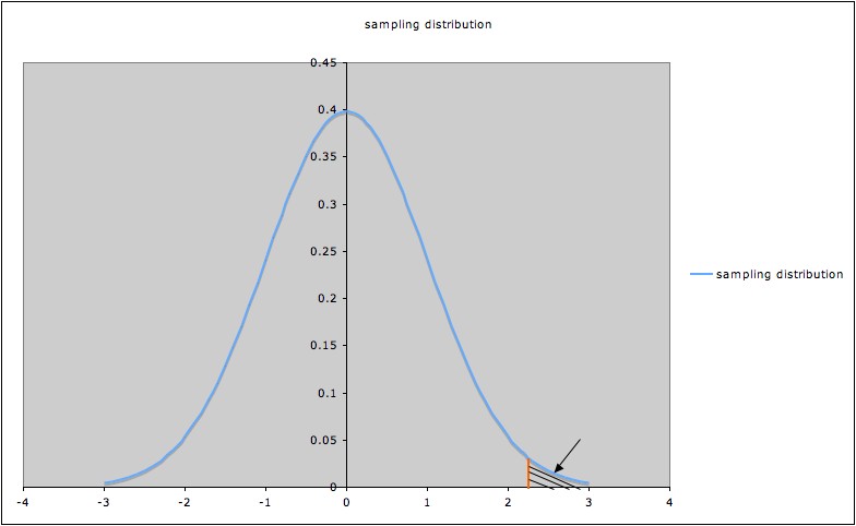
Since the shaded area indicated by the arrow is the p-value corresponding to \(t_\alpha\), that p-value (shaded area) is \(\alpha\).
To have p-value less than \(\alpha\), a t-value for this test must be to the right of \(t_\alpha\).
So the probability of rejecting the null hypothesis when it is true is the probability that \(t > t_\alpha\), which we saw above is \(\alpha\).
In other words, the probability of Type I error is \(\alpha\). \(\alpha\) is also called the bound on Type I error. Choosing a value \(\alpha\) is sometimes called setting a bound on Type I error.
The significance level \(\alpha\) is the probability of making the wrong decision when the null hypothesis is true.
Type II error
Accepting the null hypothesis when in fact the alternate hypothesis is true is called a Type II error.
Note: “The alternate hypothesis” in the definition of Type II error may refer to the alternate hypothesis in a hypothesis test, or it may refer to a “specific” alternate hypothesis.
For example: In a t-test for a sample mean \(\mu\), with null hypothesis \(\mu = 0\) and alternate hypothesis \(\mu > 0\), we may talk about the Type II error relative to the general alternate hypothesis \(\mu > 0\), or may talk about the Type II error relative to the specific alternate hypothesis \(\mu > 1\). Note that the specific alternate hypothesis is a special case of the general alternate hypothesis.
Beta
\(\beta\) is the probability of making the wrong decision when the specific alternate hypothesis is true.
- When the alternative hypothesis builds up a right tail test, \(\beta\) is \(P(X < t | h_1)\).
- When the alternative hypothesis builds up a left tail test, \(\beta\) is \(P(X > t | h_1)\).
- When the alternative hypothesis builds up a two-tail test, \(\beta\) is \(P(X < |t| | h_1)\).
Connection between Type I error and Type II error
The following diagram illustrates the Type I error and the Type II error against the specific alternate hypothesis \(\mu = 1\) in a hypothesis test for a population mean \(\mu\), with null hypothesis \(\mu = 0\), alternate hypothesis \(\mu > 0\), and significance level \(\alpha = 0.05\).
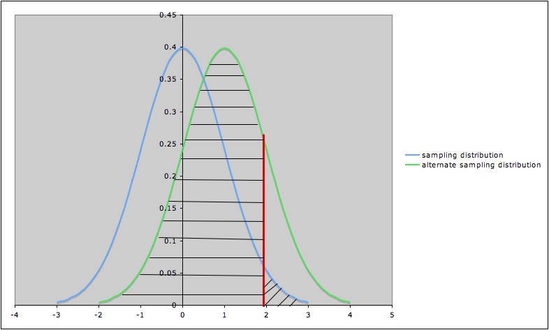
- The blue (leftmost) curve is the sampling distribution assuming the null hypothesis \(\mu = 0\)
- The green (rightmost) curve is the sampling distribution assuming the specific alternate hypothesis \(\mu = 1\)
- The vertical red line shows the cut-off for rejection of the null hypothesis: the null hypothesis is rejected for values of the test statistic to the right of the red line (and not rejected for values to the left of the red line)
- The area of the diagonally hatched region to the right of the red line and under the blue curve is the probability of type I error (\(\alpha\))
- The area of the horizontally hatched region to the left of the red line and under the green curve is the probability of Type II error (\(\beta\))
Power
The power of a statistical procedure can be thought of as the probability that the procedure will detect a true difference of a specified type.
Power is the probability that a randomly chosen sample satisfying the model assumptions will detect a difference of the specified type when the procedure is applied, if the specified difference does indeed occur in the population being studied.
Note also that power is a conditional probability: the probability of detecting a difference, if indeed the difference does exist.
As with Type II error, we need to think of power in terms of power against a specific alternative rather than against a general alternative.
- When the alternative hypothesis builds up a right tail test, power is \(P(X > t | h_1)\).
- When the alternative hypothesis builds up a left tail test, power is \(P(X < t | h_1)\).
- When the alternative hypothesis builds up a two-tail test, power is \(P(X > |t| | h_1)\).
For Example, if we are performing a hypothesis test for the mean of a population, with null hypothesis \(H_0\): \(\mu = 0\), and are interested in rejecting \(H_0\) when \(\mu > 0\), we might calculate the power of the test against the specific alternative \(H_1\): \(\mu = 1\), or against the specific alternate \(H_3\): \(\mu = 3\), etc. The picture below shows three sampling distributions:
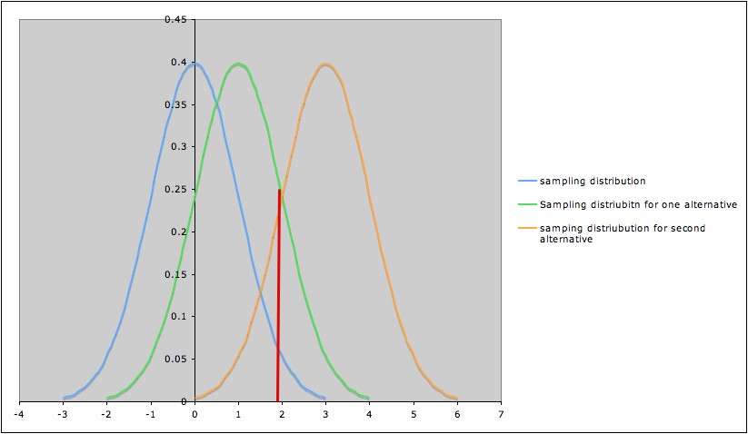
- The sampling distribution assuming \(H_0\) (blue; leftmost curve)
- The sampling distribution assuming \(H_1\) (green; middle curve)
- The sampling distribution assuming \(H_3\) (yellow; rightmost curve)
The red line marks the cut-off corresponding to a significance level \(\alpha = 0.05\).
- The area under the blue curve to the right of the red line is \(0.05\).
- The area under the green curve the to right of the red line is the probability of rejecting the null hypothesis (\(\mu = 0\)) if the specific alternative \(H_1\): \(\mu = 1\) is true. In other words, this area is the power of the test against the specific alternative \(H_1\): \(\mu = 1\). This power is greater than \(0.05\), but noticeably less than \(0.50\).
- The area under the yellow curve the to right of the red line is the power of the test against the specific alternative \(H_3\): \(\mu = 3\). This power is much larger than \(0.5\).
This illustrates the general phenomenon that the farther an alternative is from the null hypothesis, the higher the power of the test to detect it.
It is not usually possible to calculate the power against a general alternative, since the general alternative is made up of infinitely many possible specific alternatives.
Also note that, \(\text{Power} = 1 - \beta\).
