When reading some implementation of LDA, I meet the term Alias table. After some
searching, it is a family of efficient algorithms for sampling from a discrete
probability distribution, which requires \(O(n \log n)\) or \(O(n)\) time for
preprocessing, and \(O(1)\) time for generating each sample.
Directly reading Vose’s paper makes me feel a little confused, after reading this article (by Keith Schwarz), everything turns out to be very clear.
I will discuss the way to sample from known distribution step by step.
Sample from known distribution directly
Assume: we have a uniform random number generator at hand. And this assumption is hold
for whole article.
Suppose we want to sample numbers between \([0, 1)\), imagine there is a segment, and we can uniformly select points from that segment. Suppose the segment is composed with sub-segments, which are mutually disjoint with each other, the probability we select the sub-segment is proportional to its length. The longer the sub-segment, the more probably our selected point belongs to it.
There are two straight forward ways to sample from a known distribution with uniform random number generator, one is based one least common multiple, the other is based on searching with the ordered accumulated probabilities.
LCM way
Suppose the probabilities \(\{p_1, \cdots, p_n\}\) are rational numbers. Following is the description of algorithm:
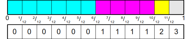
Above is an example for sampling from \(\{\frac{1}{2}, \frac{1}{3}, \frac{1}{12}, \frac{1}{12}\}\).
This algorithm requires \(O(\prod_i d_i)\) initialization time, \(\Theta(1)\) sampling time, and \(O(\prod_i d_i)\) space.
Searching way
This algorithm is also called Roulette Wheel Selection. Following is the description of algorithm:
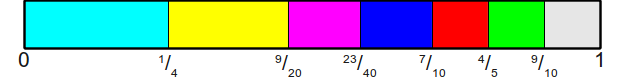
Above is an example for sampling from \(\{\frac{1}{4}, \frac{1}{5}, \frac{1}{8}, \frac{1}{8}, \frac{1}{8}, \frac{1}{10}, \frac{1}{10}, \frac{1}{10}\}\).
This algorithm requires \(\Theta(n)\) initialization time, \(\Theta(\log(n))\) sampling time, and \(\Theta(n)\) space.
It is possible to improve the expected sampling performance by building an unbalanced binary search tree, which is extremely well-studied and is called the optimal binary search tree problem. There are many algorithms for solving this problem; it is known that an exact solution can be found in time \(O(n^2)\) using dynamic programming, and there exist good linear-time algorithms that can find approximate solutions. Additionally, the splay tree data structure, a self-balancing binary search tree, can be used to get to within a constant factor of the optimal solution.
Sample from known distribution with rejection
Now, imagine we are going to sample \(n\) numbers with probabilities \(\{p_1, \cdots, p_n\}\) from a bounding box, which is composed as follows: each probability \(p_i\) builds up a rectangle with width \(w\) and height \(\max(p_i)\), then the bounding box is splitted by \(n + 1\) logic components, where \(n\) rectangle components corresponding to \(n\) probabilities, and a remaining area.
Following is an example for bounding box of probabilities \(\{\frac{1}{2}, \frac{1}{3}, \frac{1}{12}, \frac{1}{12}\}\):
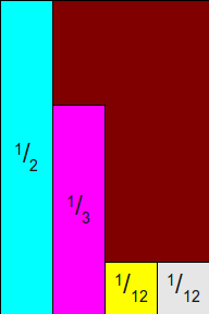
Then we sample points from the bounding box, when the sampled point belongs to the rectangle built by a probability, keep it, or discard it and keep going on sampling until getting one belongs to a rectangle.
Following is the description of algorithm:
This algorithm requires \(\Theta(n)\) initialization time, \(\Theta(\log(n))\) expected sampling time, and \(\Theta(n)\) space.
The Alias Table Method
The alias table method improves above algorithm by building up an alias table so as to avoid rejection and re-sampling in the sampling process.
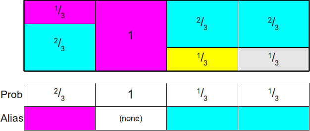
It can be shown that the height of the rectangles doesn’t impact the result. So first scale the heights of the rectangles as the probabilities with the number of probabilities, such that the total area of all the rectangles becomes \(1\). Then we rearrange the rectangles so as to build up a rectangle bounding box with area \(1\).
Following is an example for \(\{\frac{1}{2}, \frac{1}{3}, \frac{1}{12}, \frac{1}{12}\}\)
Naive Alias Table Method
The naive alias table method builds up the bounding box with a straight forward way.
Following is the description of algorithm:
It is clear that this algorithm requires \(O(n^2)\) initialization time, \(\Theta(1)\) expected sampling time, and \(\Theta(n)\) space.
Vose’s Alias Table Method
The Vose’s alias table method further improves the performance in the initialization step.
Following is the description of algorithm:
The algorithm requires \(\Theta(n)\) initialization time, \(\Theta(1)\) expected sampling time, and \(\Theta(n)\) space.
