Notes On Reinforcement Learning

Introduction of reinforcement learning

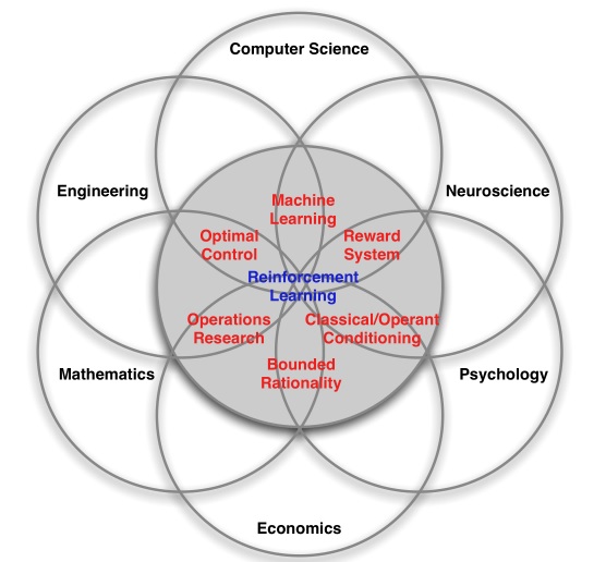
Reinforcement learning sits at the intersection of many different fields of science.

Reinforcement learning differentiates from other machine learning paradigms in following ways: there is no supervior, only a reward signal; feedback is delayed, not instantaneous; time matters (sequential, non-i.i.d data); agent’s actions affect the subsequent data it receives.

Rewards

A reward \(R_t\) is a scalar feedback signal, which indicates how well agent is doing at step \(t\). The agent’s job is to maximise cumulative reward.

Reinforcement learning is based on the reward hypothesis: all goals can be described by the maximisation of expected cumulative reward.

Agent and environment

At each step \(t\) the agent executes action \(A_t\), receives observation \(O_t\), and receives scalar reward \(R_t\). The environment receives action \(A_t\), emits observation \(O_{t+1}\), and emits scalar reward \(R_{t+1}\).

History and state

The history is the sequence of observations, actions, rewards

$$H_t = O_1, R_1, A_1, \cdots, A_{t-1}, O_t, R_t$$

According to the history, the agent selects actions and the environment selects observations/rewards. State is the information used to determine what happens next. Formally, state is a function of the history:

$$S_t = f(H_t)$$

The environment state \(S_t^e\) is the environment’s private representation. Whatever data the environment uses to pick the next observation/reward. The environment state is not usually visible to the agent. Even if \(S_t^e\) is visible, it may contain irrelevant information.

The agent state \(S_t^a\) is the agent’s internal representation. Whatever information the agent uses to pick the next action. It is the information used by reinforcement learning algorithms. It can be any function of history \(S_t^a = f(H_t)\).

Information state

An information state (a.k.a Markov state) contains all useful information from the history.

A state \(S_t\) is Markov if and only if \(P[S_{t+1}|S_t] = P[S_{t+1}|S_1,\cdots,S_t]\).

It means the future is independent of the past given the present, once the state is known, the history may be thrown away.

Fully observable environments

Agent directly observes environment state, \(O_t = S_t^a = S_t^e\). Formally, this is a Markov decision process.

Partially observable environments

Agent indirectly observes environment, the agent state is not the same as environment state. Formally this is a partially observable Markov decision process.

Agent must construct its own state representation \(S_t^a\), e.g.

• complete history: \(S_t^a = H_t\)
• beliefs of environment state: \(S_t^a = (P[S_t^e = s^1], \cdots, P[S_t^e = s^n])\)
• recurrent neural network: \(S_t^a = \delta(S_{t-1}^aW_s + O_tW_o)\)

Major components of an RL agent

An RL agent may include one or more of these compoents:

• policy: agent’s behaviour function; it is a map from state to action

  • deterministic policy: \(a = \pi(s)\)
  • stochastic policy: \(\pi(a | s) = P[A_t = a | S_t = s]\)

• value function: how good is each state and/or action; it is a prediction of future reward

  $$v_\pi(s) = E_\pi[R_{t+1} + \gamma R_{t+2} + \gamma^2 R_{t+3} + \cdots | S_t = s]$$

• model: agent’s representation of the environment; it predicts what the environment will do next

  • \(P\) predicts the next state: \(P_{ss’}^a = P[S_{t+1} = s’ | S_t = s, A_t = a]\)
  • \(R\) predicts the next (immediate) reward: \(R_s^a = E[R_{t+1} | S_t = s, A_t = a]\)

Categories of RL agents

• v1

  • value based

    • no policy (implicit)
    • value function

  • policy based

    • policy
    • no value function

  • actor critic

    • policy
    • value function

• v2

  • model free

    • policy and/or value function
    • no model

  • model based

    • policy and/or value function
    • model

Learning and planning

There are two fundamental problems in sequential decision making

• reinforcement learning:

  • the environment is initially unknown
  • the agent interacts with the environment
  • the agent improves its policy

• planning

  • a model of the environment is known
  • the agent performs computations with its model (without any external interaction)
  • the agent imporves its policy
  • a.k.a deliberation, reasoning, introspection, pondering, thought, search

Exploration and exploitation

Reinforcement learning is like trial-and-error learning, the agent should discover a good policy from its experiences of the environment without losing too much reward along the way.

Exploration finds more information about the environment. Exploitation exploits known information to maximise reward. It is usually important to explore as well as exploit.

Introduction to MDPs

Markov decision processes formally describe an environment for reinforcement learning where the environment is fully observable. Almost all RL problems can be formalised as MDPs, e.g., Optimal control primirily deals with continuous MDPs; Partially observable problems can be converted into MDPs; Bandits are MDPs with one state.

Markov process

A Markov process is a memoryless random process, i.e. a sequence of random states \(S_1\), \(S_2\), … with the Markov property.

A Markov process (or Markov chain) is a tuple \(<S, P>\)

• \(S\) is a (finite) set of states
• \(P\) is a state transition probability matrix, \(P_{ss’} = P[S_{t+1} = s’ | S_t = s]\)

Markov reward process

A Markov reward process is a Markov chain with values.

A Markov reward process is a tuple \(<S, P, R, \gamma>\)

• \(S\) is a finite set of states
• \(P\) is a state transition probability matrix, \(P_{ss’} = P[S_{t+1} = s’ | S_t = s]\)
• \(R\) is a reward function, \(R_s = E[R_{t+1} | S_t=s]\)
• \(\gamma\) is a discount factor, \(\gamma \in [0, 1]\)

Return

The return \(G_t\) is the total discounted reward from time-step \(t\)

$$G_t = R_{t+1} + \gamma R_{t+2} + \cdots = \sum_{k=0}^\infty \gamma^k R_{t+k+1}$$

The discount \(\gamma \in [0, 1]\) is the present value of future rewards. The value of receiving reward \(R\) after \(k + 1\) time-steps is \(\gamma^k R\).

Value function

The value function \(v(s)\) gives the long-term value of state \(s\). The state value function \(v(s)\) of an MDP is the expected return starting from state \(s\)

$$v(s) = E[G_t | S_t = s]$$

The value function can be decomposed into two parts: immediate reward \(R_{t+1}\) and discounted value of successor state \(\gamma v(S_{t+1})\):

$$v(s) = E[G_t | S_t = s] = E[R_{t+1} + \gamma v(S_{t+1}) | S_t = s] = R_s + \gamma \sum_{s' \in S} P_{ss'}v(s')$$

The Bellman equation can be expressed concisely using matrices,

$$v = R + \gamma Pv$$

where \(v\) is a column vector with one entry per state

$$\begin{matrix}v(1) \\ \vdots \\ v(n) \end{matrix} = \begin{matrix}R_1 \\ \vdots \\ R_n \end{matrix} + \gamma \begin{matrix}P_{11} & \cdots & P_{1_n} \\ \vdots & {} & {} \\ P_{n1} & \cdots & P_{nn} \end{matrix} \begin{matrix}v(1) \\ \vdots \\ v(n) \end{matrix}$$

The Bellman equation is a linear equation, it can be solved directly, \(v = (I - \gamma P)^{-1}R\). For \(n\) states, the computational complexity is \(O(n^3)\).

Direct solution only possible for small MRPs, for large MRPs, there are many iterative methods, e.g.

• dynamic programming
• monte-carlo evaluation
• temporal-difference learning

Markov decision process

A Markov decision process is a Markov reward process with decision. It is an environment in which all states are Markov.

A Markov decision process is a tuple \(<S, A, P, R, \gamma>\)

• \(S\) is a finite set of states
• \(A\) is a finite set of actions
• \(P\) is a state transition probability matrix, \(P_{ss’}^a = P[S_{t+1} = s’ | S_t = s, A_t = a]\)
• \(R\) is a reward function, \(R_s^a = E[R_{t+1} | S_t = s, A_t = a]\)
• \(\gamma\) is a discount factor \(\gamma \in [0, 1]\)

Policies

A policy \(\pi\) is a distribution over actions given states, \(\pi(a | s) = P[A_t = a | S_t = s]\). A policy fully defines the behaviour of an agent. MDP policies depend on the current state (not the history), i.e., policies are stationary (time-independent), \(A_t \sim \pi(\cdot | S_t), \forall t > 0\).

Given an MDP \(M = <S, A, P, R, \gamma>\) and a policy \(\pi\), the state sequence \(S_1, S_2, \cdots\) is a Markov process \(<S, P^\pi>\) and the state and reward sequence \(S_1, R_2, S_2, \cdots\) is a Markov reward process \(<S, P^\pi, R^\pi, \gamma>\) where

$$P_{ss'}^\pi = \sum_{a \in A} \pi (a | s) P_{ss'}^a \\ R_{s}^\pi = \sum_{a \in A} \pi (a | s) R_s^a$$

Value function

The state-value function \(v_\pi(s)\) of an MDP is the expected return starting from state \(s\), and then following policy \(\pi\), \(v_\pi(s) = E_\pi [G_t | S_t = s]\).

The state-value function can again be decomposed into immediate reward plus discounted value of successor state,

$$\begin{array} {}v_\pi(s) &=& E_\pi [R_{t+1} + \gamma v_\pi(S_{t+1}) | S_t = s] \\ &=& \sum_{a \in A} \pi(a | s) q_\pi(s, a) \\ &=& \sum_{a \in A} \pi(a | s) \left(R_s^a + \gamma\sum_{s' \in S} P_{ss'}^a v_\pi(s')\right) \end{array}$$

The action-value function \(q_\pi(s, a)\) is the expected return starting from state \(s\), taking action \(a\), and then following policy \(\pi\), \(q_\pi(s, a) = E_\pi [G_t | S_t = s, A_t = a]\).

The action-value function can be decomposed,

$$\begin{array} {}q_\pi(s, a) &=& E_\pi [R_{t+1} + \gamma q_\pi(S_{t+1}, A_{t+1}) | S_t = s, A_t = a] \\ &=& R_s^a + \gamma \sum_{s' \in S} P_{ss'}^a v_\pi(s') \\ &=& R_s^a + \gamma \sum_{s' \in S}P_{ss'}^a\sum_{a' \in A}\pi(a'|s')q_\pi(s', a') \end{array}$$

Optimal value function

The optimal state-value function \(v_*(s)\) is the maximum value function over all policies \(v_*(s) = \max_\pi v_\pi(s)\).

The optimal action-value function \(q_*(s, a)\) is the maximum action-value function over all policies \(q_*(s, a) = \max_\pi q_\pi(s, a)\).

The optimal value function specifies the best possible performance in the MDP.

Optimal policy

Define a partial ordering over policies \(\pi \geq \pi ‘ \text{ if } v_\pi(s) \geq v_{\pi ‘}(s), \forall s\)

For any Markov decision process, there exists an optimal policy \(\pi_*\) that is better than or equal to all other policies, \(\pi_* \geq \pi, \forall \pi\). All optimal policies achieve the optimal value function, \(v_{\pi_*}(s) = v_*(s)\). All optimal policies achieve the optimal action-value function, \(q_{\pi_*}(s, a) = q_*(s, a)\).

An optimal policy can be found by maximising over \(q_*(s, a)\),

$$\pi_*(a | s) = \begin{cases} 1 \text{ if } a = \arg\max_{a \in A} q_*(s, a)\\ 0 \text{ otherwise} \end{cases}$$

The optimal value functions are recursively related by the Bellman optimality equations:

$$v_*(s) = \max_a q_*(s, a) \\ q_*(s, a) = R_s^a + \gamma\sum_{s' \in S}P_{ss'}^a v_*(s') \\ v_*(s) = \max_a R_s^a + \gamma \sum_{s' \in S} P_{ss'}^a v_*(s') \\ q_*(s, a) = R_s^a + \gamma \sum_{s' \in S} P_{ss'}^a \max_{a'} q_*(s', a')$$

The Bellman optimality equation is non-linear, there is no closed form solution in general. There are many iterative solution methods, such as value iteration, policy iteration, q-learning, SARSA.

Extensions to MDPs

The following extensions are all possible:

• coutably infinite state and/or action spaces; straightforward
• continuous state and/or action spaces; closed form for linear quadratic model (LQR)

• continuous time

  • requires partial differential equations
  • Hamilton-Jacobi-Bellman (HJB) equation
  • limiting case of Bellman equation as time-step -> 0

Partially observable MDPs

A partially observable Markov decision process is an MDP with hidden states. It is a hidden Markov model with actions. A POMDP is a tuple \(<S, A, O, P, R, Z, \gamma>\)

• \(S\) is a finite set of states
• \(A\) is a finite set of actions
• \(O\) is a finite set of observations
• \(P\) is a state transition probability matrix, \(P_{ss’}^a = P[S_{t+1} = s’ | S_t = s, A_t = a]\)
• \(R\) is a reward function, \(R_s^a = E[R_{t+1} | S_t = s, A_t = a]\)
• \(Z\) is an observation function, \(Z_{s’o}^a = P[O_{t+1} = o | S_{t+1} = s’, A_t = a]\)
• \(\gamma\) is a distount factor \(\gamma \in [0, 1]\)

A history \(H_t\) is a sequence of actions, observations and rewards, \(H_t = A_0, O_1, R_1, \cdots, A_{t-1}, O_t, R_t\).

A belief state \(b(h)\) is a probability distribution over states, conditioned on the history \(h\), \(b(h) = (P[S_t = s^1 | H_t = h], \cdots, P[S_t = s^n | H_t = h])\).

The history \(H_t\) satisfies the Markov property. The belief state \(b(H_t)\) satisfies the Markov property. A POMDP can be reduced to an (infinite) history tree. A POMDP can be reduced to an (infinite) belief state tree.

Average reward MDPs

An ergodic Markov process is

• recurrent: each state is visited an infinite number of times
• aperiodic: each state is visited without any systematic period

An ergodic Markov process has a limiting stationary distribution \(d^\pi(s)\) with the property \(d^\pi(s) = \sum_{s’ \in S}d^\pi(s’)Ps’s\).

An MDP is ergodic if the Markov chain induced by any policy is ergodic. For any policy \(\pi\), an ergodic MDP has an average reward per time-step \(\rho^\pi\) that is independent of start state.

$$\rho^\pi = \lim_{T \rightarrow \infty} \frac{1}{T} E[\sum_{t=1}^T R_t]$$

The value function of an undiscounted, ergodic MDP can be expressed in terms of average reward. \(\tilde{v}_\pi(s)\) is the extra reward due to starting from state \(s\), \(\tilde{v}_\pi(s) = E_\pi [\sum_{k=1}^\infty (R_{t+k} - \rho^\pi) | S_t = s]\).

Dynamic programming

Dynamic programming is used for planning in an MDP, it assumes full knowledge of the MDP.

Policy evaluation

To evaluate a given policy \(\pi\), iteratively apply the Bellman expectation backup. For synchronous backups, it follows:

• at each iteration \(k + 1\)
• for all states \(s \in S\)
• update \(v_{k+1}(s)\) from \(v_k(s’)\)
• where \(s’\) is a successor state of \(s\)

Policy iteration

Given a policy \(\pi\)

• evaluate the policy \(\pi\), \(v_\pi(s) = E[R_{t+1} + \gamma R_{t+2} + \cdots | S_t = s]\)
• improve the policy by acting greedily with respect to \(v_\pi\), \(\pi ‘ = \text{greedy}(v_\pi)\)

For a deterministic policy, \(a = \pi(s)\), we can improve the policy by acting greedily \(\pi ‘ (s) = \arg\max_{a \in A} q_\pi(s, a)\). This improves the value from any state \(s\) over one step,

$$q_\pi (s, \pi '(s)) = \max_{a \in A} q_\pi (s, a) \geq q_\pi (s, \pi(s)) = v_\pi(s)$$

It therefore improves the value function, \(v_{\pi ‘}(s) \geq v_\pi(s)\),

$$\begin{array} {}v_\pi(s) &\leq& q_\pi(s, \pi ' (s)) = E_{\pi '}[R_{t+1} + \gamma v_\pi (S_{t+1}) | S_t = s] \\ &\leq& E_{\pi '}[R_{t+1} + \gamma q_\pi(S_{t+1}, \pi ' (S_{T+1})) | S_t = s] \\ &\leq& E_{\pi '}[R_{t+1} + \gamma R_{t+2} + \gamma^2 q_\pi (S_{t+2}, \pi ' (S_{t+2})) | S_t = s] \\ &\leq& E_{\pi '}[R_{t+1} + \gamma R_{t+2} + \cdots | S_t = s] = v_{\pi '}(s) \end{array}$$

If improvements stop, \(q_\pi (s, \pi ‘ (s)) = \max_{a \in A} q_\pi (s, a) = q_\pi (s, \pi(s)) = v_\pi(s)\), then the Bellman optimality equation has been satisfied \(v_\pi(s) = \max_{a \in A} q_\pi(s, a)\).

Value iteration

Any optimal policy can be subdivided into two components, an optimal first action \(A_*\), and followed by an optimal policy from successor state \(S’\).

If we know the solution to subproblems \(v_*(s’)\), then solution \(v_*(s)\) can be found by one-step lookahead

$$v_*(s) \leftarrow \max_{a \in A} R_s^a + \gamma \sum_{s' \in S} P_{ss'}^a v_*(s')$$

The idea of value iteration is to apply these updates iteratively starting with final rewards and working backwards.

Monte-Carlo learning

MC methods are model-free (no knowledge of MDP transitions/rewards) and learn directly from complete episodes (no bootstrapping). It uses the simplest possible idea: value = mean return. The caveat is MC methods require all episodes must terminate.

Incremental Monte-Carlo updates

To update \(V(s)\) incrementally after episode \(S_1, A_1, R_2, \cdots, S_T\), for each state \(S_t\) with return \(G_t\)

• \(N(S_t) \leftarrow N(S_t) + 1\)
• \(V(S_t) \leftarrow V(S_t) + \frac{1}{N(S_t)}(G_t - V(S_t))\)

In non-stationary problems, it can be useful to track a running mean, i.e. forget old episodes

$$V(S_t) \leftarrow V(S_t) + \alpha(G_t - V(S_t))$$

Temporal-Difference learning

TD methods are model-free and learn directly from incomplete episodes by bootstrapping.

The simplest TD learning algorithm TD(0) updates value \(V(S_t)\) toward estimated return \(R_{t+1} + \gamma V(S_{t+1})\)

$$V(S_t) \leftarrow V(S_t) + \alpha (R_{t+1} + \gamma V(S_{t+1}) - V(S_t))$$

where \(R_{t+1} + \gamma V(S_{t+1})\) is called the TD target, \(\delta_t = R_{t+1} + \gamma V(S_{t+1}) - V(S_t)\) is called the TD error.

Certainty equivalence

MC converges to solution with minimum mean-squared error, it gives the best fit to the observed returns

$$\sum_{k = 1}^K \sum_{t = 1}^{T_k} (G_t^k - V(s_t^k))^2$$

TD(0) converges to solution of max likelihood Markov model. Solution to the MDP \(<S, A, \tilde{P}, \tilde{R}, \gamma>\) that best fits the data

$$\tilde{P}_{s,s'}^a = \frac{1}{N(s, a)} \sum_{k = 1}^K \sum_{t = 1}^{T_k} 1 (s_t^k, a_t^k, s_{t+1}^k = s, a , s') \\ \tilde{R}_s^a = \frac{1}{N(s, a)} \sum_{k = 1}^K \sum_{t = 1}^{T_k} 1 (s_t^k, a_t^k = s, a) r_t^k$$

TD exploits Markov property, thus usually more efficient in Markov environments; MC does not exploit Markov property, thus usually more effective in non-Markov environments.

\(TD(\lambda)\)

The \(\lambda\text{-return} G_t^\lambda\) combines all n-step return \(G_t^{(n)}\), using weight \((1 - \lambda)\lambda^{n - 1}\), \(G_t^\lambda = (1 - \lambda)\sum_{n = 1}^\infty \lambda^{n - 1}G_t^{(n)}\).

Forward-view \(TD(\lambda)\) updates \(V(S_t) \leftarrow V(S_t) + \alpha(G_t^\lambda - V(S_t))\).

Backward-view \(TD(\lambda)\) keeps an eligibility trace for every state \(s\), updates value \(V(s)\) for every state \(s\) in proportion to TD-error \(\delta_t\) and eligibility trace \(E_t(s)\)

$$\delta_t = R_{t+1} + \gamma V(S_{t+1}) - V(S_t) \\ V(s) \leftarrow V(s) + \alpha\delta_t E_t (s)$$

When \(\lambda = 0\), only the current state is updated, it is equivalent to TD(0). When \(\lambda = 1\), credit is deferred until end of episode, it is the same as total update for MC. The difference is that in TD(1) the error is accumulated online, step-by-step.

Offline and online updates

Offline updates are accumulated within episode but applied in batch at the end of episode.

Online updates are applied online at each step within episode.

Model-free control

On-policy learning learns about policy \(\pi\) from experience sampled from \(\pi\). Off-policy learning learns about policy \(\pi\) from experience sampled from \(\mu\).

On-policy Monte-Carlo control

Greedy policy improvement over \(V(s)\) requires model of MDP

$$\pi ' (s) = \arg\max_{a \in A} R_s^a + P_{ss'}^a V(s')$$

Greedy policy improvement over \(Q(s, a)\) is model-free

$$\pi ' (s) = \arg\max_{a \in A} Q(s, a)$$

\(\epsilon\text{-Greedy}\) exploration with probability \(1 - \epsilon\) choose the greedy action; with probability \(\epsilon\) choose an action at random

$$\pi(a|s) = \begin{cases} \frac{\epsilon}{m} + 1 - \epsilon \text{ if } a^* = \arg\max_{a \in A} Q(s, a) \\ \frac{\epsilon}{m} \text{ otherwise} \end{cases}$$

For any \(\epsilon\text{-Greedy}\) policy \(\pi\), the \(\epsilon\text{-Greedy}\) policy \(\pi ‘\) with respect to \(q_\pi\) is an improvement, \(v_{\pi ‘}(s) \geq v_\pi(s)\)

$$\begin{array} {}q_\pi(s, \pi '(s)) &=& \sum_{a \in A} \pi ' (a|s) q_\pi (s, a) \\ &=& \frac{\epsilon}{m} \sum_{a \in A} q_\pi(s, a) + (1 - \epsilon) \max_{a \in A} q_\pi (s, a) \\ &\geq& \frac{\epsilon}{m} \sum_{a \in A} q_\pi (s, a) + (1 - \epsilon) \sum_{a \in A} \frac{\pi(a|s) - \frac{\epsilon}{m}}{1 - \epsilon} q_\pi (s, a) \\ &=& \sum_{a \in A} \pi(a|s)q_{\pi}(s, a) = v_\pi (s) \end{array}$$

Therefore from policy improvement theorem, \(v_{\pi ‘}(s) \geq v_\pi(s)\).

Greedy in the limit with infinite exploration

All state-action pairs are explored infinitely many times \(\lim_{k \rightarrow \infty} N_k(s, a) = \infty\). The policy converges on a greedy policy, \(\lim_{k \rightarrow \infty} \pi_k(a|s) = 1(a = \arg\max_{a’ \in A} Q_k(s, a’))\).

Sample k-th episode using \(\pi\): \(\{S_1, A_1, R_2, \cdots, S_t\} \sim \pi\), for each state \(S_t\) and action \(A_t\) in the episode,

$$N(S_t, A_t) \leftarrow N(S_t, A_t) + 1 \\ Q(S_t, A_t) \leftarrow Q(S_t, A_t) + \frac{1}{N(S_t, A_t)}(G_t - Q(S_t, A_t))$$

Improve policy based on new action-state function

$$\epsilon \leftarrow \frac{1}{k} \\ \pi \leftarrow \epsilon\text{-greedy}(Q)$$

On-policy temporal-difference learning

Use TD instead of MC in the control loop, s.t. apply TD to \(Q(S, A)\) and use \(\epsilon\text{-greedy}\) policy improvement and update every time step.

$$Q(S, A) \leftarrow Q(S, A) + \alpha(R + \gamma Q(S', A') - Q(S, A))$$

Similr to TD, there also exits \(SARSA(\lambda)\).

Off-policy learning

Off-policy learning evaluate target policy \(\pi(a | s)\) to compute \(v_\pi(s)\) or \(q_\pi(s, a)\) while following behaviour policy \(\mu(a | s)\)

$$\{S_1, A_1, R_2, \cdots, S_t\} \sim \mu$$

To use importance sampling for off-policy Monte-Carlo, use returns generated from \(\mu\) to evaluate \(\pi\), weight return \(G_t\) according to similarity between policies, multiply importance sampling corrections along whole episode and update value towards corrected return. Cannot use if \(\mu\) is zero when \(\pi\) is non-zero. Importance sampling can dramatically increase variance.

Q-learning

We now consider off-policy learning of action-values \(Q(s, a)\), no importance sampling is required. With importance sampling, next action is chosen using behaviour policy \(A_{t+1} \sim \mu(\cdot | S_t)\). But we consider alternative successor action \(A’ \sim \pi(\cdot | S_t)\) and update \(Q(S_t, A_t)\) towards value of alternative action

$$Q(S_t, A_t) \leftarrow Q(S_t, A_t) + \alpha(R_{t+1} + \gamma Q(S_{t+1}, A') - Q(S_t, A_t))$$

We now allow both behaviour and target policies to improve. The target policy \(\pi\) is greedy w.r.t. \(Q(s, a)\)

$$\pi(S_{t+1}) = \arg\max_{a'} Q(S_{t+1}, a')$$

The behaviour policy \(\mu\) is e.g. \(\epsilon\text{-greedy}\) w.r.t. \(Q(s, a)\), the Q-learning target then simplifies

$$\begin{array} {}R_{t+1} + \gamma Q(S_{t+1}, A') &=& R_{t+1} + \gamma Q(S_{t+1}, \arg\max_{a'} Q(S_{t+1}, a')) \\ &=& R_{t+1} + \max_{a'} \gamma Q(S_{t+1}, a') \end{array}$$

The update is

$$Q(S, A) \leftarrow Q(S, A) + \alpha (R + \gamma \max_{a'} Q(S', a') - Q(S, A))$$

Relationship between DP and TD

Note: in below equations, \(x \overset{\alpha}\leftarrow y \equiv x \leftarrow x + \alpha(y - x)\)

$$\begin{cases} \text{Iterative Policy Evaluation } V(s) \leftarrow E[R + \gamma V(S') | s] \\ \text{TD learning } V(s) \overset{\alpha}{\leftarrow} R + \gamma V(s') \end{cases}$$ $$\begin{cases} \text{Q-Policy Iteration } Q(s, a) \leftarrow E[R + \gamma Q(S', A') | s, a] \\ \text{SARSA } Q(S, A) \overset{\alpha}{\leftarrow} R + \gamma Q(S', A') \end{cases}$$ $$\begin{cases} \text{Q-Value Iteration } Q(s, a) \leftarrow E[R + \gamma \max_{a' \in A} Q(S', a') | s, a] \\ \text{Q-Learning } Q(S, A) \overset{\alpha}{\leftarrow} R + \gamma \max_{a' \in A} Q(S', A') \end{cases}$$

Value function approximation

For large MDPs, there are too many states and/or actions to store in memory. It is slow to learn the value of each state individually. So we estimate value function with function approximation

$$\hat{v}(s, w) \approx v_\pi (s) \\ \text{or } \hat{q}(s, a, w) \approx q_\pi(s, a)$$

and generalise from seen states to unseen states, and update parameter \(w\) using MC or TD learning.

In RL, there is no supervisor, only rewards, thus we don’t have true value function \(v_\pi (s)\). In practice, we substitute a target for \(v_\pi(s)\),

• For MC, the target is the return \(G_t\)
• For TD(0), the target is the TD target \(R_{t+1} + \gamma \hat{v} (S_{t+1}, w)\)
• For \(TD(\lambda)\), the target is the \(\lambda\text{-return} G_t^\lambda\)

We can also approximate the action-value function

$$\hat{q}(S, A, w) \approx q_\pi(S, A)$$

Deep Q-networks

Gradient descent is simple and appealing but it is not sample efficient. Batch methods seek to find the best fitting value function given the agent’s experience (training data).

Given value function approximation \(\hat{v}(s, w) \approx v_\pi (s)\), and experience \(D\) consisting of <state, value> pairs

$$D = \{<s_1, v_1^\pi>, <s_2, v_2^\pi>, \cdots, <s_T, v_T^\pi>\}$$

Least squares algorithms find parameter vector \(w\) minimising sum-squared error between \(\hat{v}(s_t, w)\) and target values \(v_t^\pi\),

$$\begin{array} LS(w) &=& \sum_{t=1}^T(v_t^\pi - \hat{v}(s_t, w))^2 \\ &=& E_D[(v^\pi - \hat{v}(s, w))^2] \end{array}$$

DQN uses experience replay and fixed Q-targets

• take action \(a_t\) according to \(\epsilon\text{-greedy}\) policy
• store transition \((s_t, a_t, r_{t+1}, s_{t+1})\) in replay memory \(D\)
• sample random mini-batch of transitions \((s, a, r, s’)\) from \(D\)
• compute Q-learning targets w.r.t. old, fixed parameters \(w^-\)
• optimise MSE between Q-network and Q-learning targets, \(L_i(w_i) = E_{s, a, r, s’ \sim D_i} [(r + \gamma \max_{a’} Q(s’, a’; w_i^-) - Q(s, a; w_i))^2]\)
• using variant of stochastic gradient descent

Model-free policy gradient

Policy-based RLs have better convergence properties, are effective in high-dimensional or continuous action spaces. And it is possible to learn stochastic policies. The disadvantages of policy-based RLs are that they typically converge to a local rather than global optimum and evaluating a policy is typically inefficient and high variance.

Score function

To compute the policy gradient analytically, assume policy \(\pi_\theta\) is differentiable whenever it is non-zero and we know the gradient \(\nabla_\theta\pi_\theta(s,a)\), the likelihood ratios exploit the following identity

$$\begin{array} {}\nabla_\theta\pi_\theta(s, a) &=& \pi_\theta(s, a)\frac{\nabla_\theta\pi_\theta(s, a)}{\pi_\theta(s, a)} \\ &=& \pi_\theta(s, a)\nabla_\theta\log\pi_\theta(s, a) \end{array}$$

The score function is \(\nabla_\theta\log\pi_\theta(s, a)\).

Monte-Carlo policy gradient

Using parameters by stochastic gradient ascent, using policy gradient theorem, using return \(v_t\) as an unbiased sample of \(Q^{\pi_\theta}(s_t, a_t)\)

$$\Delta\theta_t = \alpha\nabla_\theta\log\pi_\theta(s_t,a_t)v_t$$

Actor-critic policy gradient

Monte-Carlo policy gradient still has high variance, we use a critic to estimate the action-value function, \(Q_w(s, a) \approx Q^{\pi_\theta}(s,a)\). Actor-critic algorithms maintain two sets of parameters

• critic: updates action-value function parameters \(w\)
• actor: updates policy parameters \(\theta\), in direction suggested by critic

Actor-critic algorithms follow an approximate policy gradient

$$\nabla_\theta J(\theta) \approx E_{\pi_\theta}[\nabla_\theta\log\pi_\theta(s, a)Q_w(s, a)] \\ \Delta\theta = \alpha\nabla_\theta\log\pi_\theta(s, a)Q_w(s, a)$$

Summary of policy gradient algorithms

$$\begin{array} {}\nabla_\theta J(\theta) &=& E_{\pi_\theta} [\nabla_\theta\log\pi_\theta(s, a) v_t] &\text{ reinforce} \\ &=& E_{\pi_\theta} [\nabla_\theta\log\pi_\theta(s, a) Q^w(s, a)] &\text{ Q actor-critic} \\ &=& E_{\pi_\theta} [\nabla_\theta\log\pi_\theta(s, a) A^w(s, a)] &\text{ Advantage actor-critic} \\ &=& E_{\pi_\theta} [\nabla_\theta\log\pi_\theta(s, a) \delta] &\text{ TD actor-critic} \\ &=& E_{\pi_\theta} [\nabla_\theta\log\pi_\theta(s, a) \delta e] &\text{ TD(}\lambda\text{) actor-critic} \\ G_\theta^{-1}\nabla_\theta J(\theta) &=& w &\text{ Natural actor-critic} \end{array}$$

Model-based reinforcement learning

A model \(M\) is a representation of an MDP \(<S, A, P, R>\), parameterized by \(\eta\). Assuming state space \(S\) and action space \(A\) are known, a model \(M=<P_\eta, R_\eta>\) represents state transitions \(P_n \approx P\) and rewards \(R_\eta \approx R\)

$$S_{t+1} \sim P_\eta(S_{t+1} | S_t, A_t) \\ R_{t+1} = R_\eta(R_{t+1} | S_t, A_t)$$

Typically we assume conditional independence between state transitions and rewards \(P[S_{t+1}, R_{t+1} | S_t, A_t] = P[S_{t+1} | S_t, A_t]P[R_{t+1} | S_t, A_t]\).

Model learning is to estimate model \(M_\eta\) from experience \(\{S_1, A_1, R_2, \cdots, S_T\}\), which is a supervised learning problem, \(S_t, A_t \rightarrow R_{t+1}, S_{t+1}\). Learning \(s, a \rightarrow r\) is a regression problem. Learning \(s, a \rightarrow s’\) is a density estimation problem.

Planning with a model is to solve the MDP \(<S, A, P_\eta, R_\eta>\) given a model \(M_\eta = <P_\eta, R_\eta>\) by using planning algorithms: value iteration, policy iteration, tree search, etc.

Sample-based planning is to use the model only to generate samples, sample experience from model

$$S_{t+1} \sim P_\eta (S_{t+1} | S_t, A_t) \\ R_{t+1} = R_\eta(R_{t+1} | S_t, A_t)$$

and apply model-free RL to samples, e.g. Monto-Carlo control, SARSA, Q-learning. Sample-based planning methods are often more efficient.

Dyna

Consider two sources of experience, real experience which is sampled from environment (true MDP) with \(S’ \sim P_{ss’}^a\) and \(R = R_s^a\); simulated experience which is sampled from model (approximate MDP) with \(S’ \sim P_\eta(S’ | S, A)\) and \(R = R_\eta(R | S, A)\).

Model-free RL has no model and learns value function (and/or policy) from real experience. Model-based RL (using sample-based planning) learns a model from real experience and plan value function (and/or policy) from simulated experience. Dyna learns a model from real experience and learns and plans value function (and/or policy) from real and simulated experience.

Simulation-based search

Forward search algorithms select the best action by lookahead. They build a search tree with the current state \(s_t\) at the root, and use a model of the MDP to look ahead. Forward search paradigm using sample-based planning, simulate episodes of experience from now with the model, and apply model-free RL to simulated episodes.

Given a model \(M_v\), Monte-Carlo tree search simulate \(K\) episodes from current state \(s_t\) using current simulation policy \(\pi\)

$$\{s_t, A_t^k, R_{t+1}^k, R_{t+1}^k, S_{t+1}^k, \cdots, S_T^k\}_{k = 1}^K \sim M_{v,\pi}$$

and build a search tree containing visited states and actions. MCTS evaluate states \(Q(s, a)\) by mean return of episodes from \(s, a\)

$$Q(s, a) = \frac{1}{N(s, a)}\sum_{k=1}^K\sum_{u=t}^T 1(S_u, A_u = s, a)G_u \overset{P}{\rightarrow} q_\pi(s, a)$$

After search is finished, select current (real) action with maximum value in search tree \(a_t = \arg\max_{a \in A} Q(s_t, a)\).

In MCTS, the simulation policy \(\pi\) improves. In each simulation, there consist of two phases (in-tree, out-of-tree)

• tree policy (improves): pick actions to maximise \(Q(S, A)\)
• default policy (fixed): pick actions randomly

In each repeat (each simulation)

• evaluate states \(Q(S, A)\) by Monte-Carlo evalution
• improve tree policy, e.e. by \(\epsilon\text{-greedy}(Q)\)

And MCTS applies Monte-Carlo control to simulated experience. It converges on the optimal search tree, \(Q(S, A) \rightarrow q_*(S, A)\).

The advantages of MC tree search are listed as follows:

• highly selective best-first search
• evaluates states dynamically (unlike DP)
• uses sampling to break curse of dimensionality
• works for black-box models (only requires samples)
• computationally efficient, anytime, parallelisable

Temporal-difference search uses TD instead of MC (bootstrapping). TD search applies SARSA to sub-MDP from now, while MC tree search applies MC control to sub-MDP from now.

TD search simulates episodes from current (real) state \(s_t\). It estimates action-value function \(Q(s, a)\). For each step of simulation, update action-values by SARSA

$$\Delta Q(S, A) = \alpha (R + \gamma Q(S', A') - Q(S, A))$$

TD search selects actions baed on action-value \(Q(s, a)\), e.g. \(\epsilon\text{-greedy}\), it may also use function approximation for \(Q\).

In Dyna-2, the agent stores two sets of feature weights, long-term memory and short-term (working) memory. Long-term memoy is updated from real experience using TD learning, general domain knowledge that applies to any episode. Short-term memory is updated from simulated experience using TD search, specific local knowledge about the current situation. Over value function is a sum of long-term and short-term memories.

Exploration and exploitation

Online decision-making involves a fundamental choice: exploitation, make the best decision given current information; exploration, gather more information. The best long-term strategy may involve short-term sacrifices. Gather enough information to make the best overall decisions.

Multi-armed bandit

A multi-armed bandit is a tuple \(<A, R>\), where \(A\) is a known set of \(m\) actions and \(R^a(r) = P[r|a]\) is an unknown probability distribution over rewards. At each step \(t\) the agent selects an actioin \(a_t \in A\), and the environment generates a reward \(r_t \sim R^{a_t}\). The goal is to maximise cumulative reward \(\sum_{\tau=1}^t r_\tau\).

The action-value is the mean reward for action \(a\), \(Q(a) = E[r | a]\). The optimal value \(V^*\) is \(V^* = Q(a^*) = \max_{a \in A} Q(a)\). The regret is the opportunity loss for one step \(l_t = E[V^* - Q(a_t)]\). The total regret is the total opportunity loss \(L_t = E[\sum_{\tau = 1}^t V^* - Q(a_\tau)]\).